Experiments & Results

1. Methods
To generate data for each experiment, as all input variables are joint angles, I created a vector of uniformly distributed random numbers with each scaled to be between in the range [0, 2*PI]. These vectors are then fed to the respective models to generate observed torques.
2. Preliminary Experiments:
I performed 2 initial parameter estimation experiments using a pendulum model and a two link planar manipulator model to test out the optimization machinery.
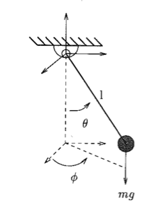
Pendulum (exp1_pendulum_calibration.py)
Two-link Planar Manipulator (exp2_two_link_calibration.py)
In the pendulum case, I generated 1000 samples from a model where the mass is 10 kg and the rope length is 30 meters. The optimization procedure was initialized with the starting mass to as 13.0 kg, and the length of the cable as 33.0 meters. Using the NCQG solver, the final solution converged on a solution with the mass being 10.21 kg and the cable length 29.68 meters. This took 425 seconds. Emboldened by the success I investigated the case of a more complicated two link manipulator.
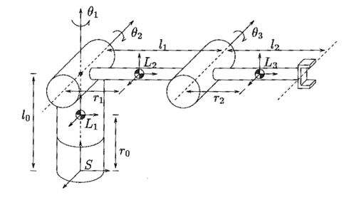
In the two link planar manipulator case the solution was generated from a model assuming the following parameters:
m1 m2 l1 l2 w1 w2 r1 r2
[5.0, 6.0, 3.0, 3.0, .3, .3, 1.5, 1.5]
Where m’s denote masses, l’s link lengths, w’s widths and r the distance to the center of mass. Strictly speaking, r = l/2, as the center of mass should coincide with the halfway point. NCQG ran starting with the point:
[5.0, 6.0, 3.3, 2.7, .28, .33, 1.1, 1.9]
After 675 seconds this converged to
[4.7 5.5 3.1 2.8, -1.5 1.1 1.6 1.6]
The objective function in this case was reduced to 0.026 from 0.0297. In this case it seemed like the solution fell down a local minima as the width for link 1 was driven to -1.5 from it’s starting point of .28. Another confounded effect is that between l1, l2 and r1, r2. However, those parameters seem to have remained stable in this case.
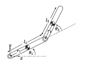
3. Three Link Manipulator (exp3_three_link.py)
There are numerous parameters for the 3 link case. The dynamics equations, due to the link geometries simplified to the following parameters:
r1 m1 w1 r2 m2 w2 h2 l3 m3 w3 h3
[.5, 0.7, 0.8, 0.5, 0.7, 0.8, 0.2, 1.0, 0.7, 0.8, 0.2]
Learning from the two link case, the link length parameters for links 1 and 2 were eliminated by using 2r=l. For link 3 as r3 canceled out in the dynamics equation, I retained the variable l3. With this setup, I performed 3 experiments:
Experiment 1: Effects of Sample Size on Accuracy
L2 Distance (from true solution)
.66
.34
.40
.39
.43
.40
.48
.38
.42
.44
Sample Size
500
1000
1500
2000
2500
3000
4000
5000
6000
7000
Time (s)
123
218
315
430
515
606
782
978
1181
1476
In terms of L2 distance, the results are a little bit depressing, however, the objective function tend to start out extremely high, 39466 for the 7000 samples case, and was driven to near zero (3.51E-11). This indicates that there might still be parameters in the model that are extraneous allowing more than one sets of inertial parameters to fit the data. As for the effect of sampling size, it seems that uniform randomly sampling the space of joint angle might be a fairly good strategy as even though the dynamics function itself is non-linear itself involving cosines and sines, the dynamics parameters themselves do not pass through any sines or cosines. In fact, the highest power term involving the unknowns are cubics.
Experiment 2: Effects of Observation Noise
I added random Gaussian noise of varying standard deviations to the torques recorded to test resilience to observation noise. However, the results are a flawed as the magnitude of noise shown here is probably not on the same order as generated torques. In addition, noise in the observation of the joint velocities and acceleration have not been considered. Each optimization ran using 1000 samples.
Experiment 3: Effects of Different Initialization Points
L2 Distance
0.44
0.50
0.46
0.40
0.46
STD
0.1
0.2
0.3
0.4
0.5
To generate the different starting points, I added uniform random noise in the range [0,5] to the ideal parameters. Using these corrupted parameters, I ran the optimization for using 1000 samples. From these results it seems clear that there are many local minimas but due to the redundancy in the dynamics parameters each one seems equal good as they can all fit the data extremely well.
3. Conclusion
Even after setting tying some of the parameters to each other, for the 3 link manipulator, there still seems to be redundant parameters leading to different dynamic models that exhibit similar dynamical characteristics. As with other issues such as determining the kinematics degrees of freedom, the parameters that needs to be tied together might depend on the configurations of the links with respect to each other. With some of the parameters, this dependence on the configuration can readily be seen. In the planar 2-link case, all of the height parameters for the rectangular prism disappeared as the robot only moves in a plane. For the spatial 3 link case the height parameter was canceled out. Practically, if two models predict the same dynamics and both works in terms of the data it seems difficult to designate one set of parameters as being the “correct” set.
L2 Distance (from true solution)
0.42
16.7
0.19
8.48
0.58
Starting Distance
9.46
16.9
8.82
13.3
10.8
Objective
5.9E-11
8.16E-12
8.90E-11
4.17E-12
6.01E-11
