- the components of the DataScribe
- introducing foreign data into IRIS Explorer
- using data elements in a template
- working with binary files
- working with arrays and lattice structures
- creating conversion scripts from templates
- creating a module control panel for the DataScribe module
- tracking errors
Overview
The DataScribe is a utility for converting users' ASCII and binary data
into and out of the IRIS Explorer lattice data type. ASCII data must be in
the form of
scalars
and/or
arrays. A scalar is a single data item, and an array is a structured
matrix of points forming a lattice. You can convert data into and out of IRIS
Explorer lattice format by building a data conversion
script
in the DataScribe.
The script is a file consisting of
input
and
output templates
and their wiring. The templates contain information, in the form of
glyphs, about the data types that you want to convert. Glyphs are
icons that represent each data type and its components in visual form. The
wiring connections map an input data type to its output data type. For
example, you may have arrays in an ASCII file that you want to bring into
IRIS Explorer. The glyphs in the input template represent the type of array
you have (such as 2D or 3D), and those in the output template indicate how
you want your array data to appear in IRIS Explorer. For example, you can
select a small, interesting section from a large and otherwise uninteresting
array by connecting input and output glyphs so that only the data you want is
converted into the IRIS Explorer lattice.
Once the script file has been set up, you can create a control panel for
it and save it as a module. You then set up a map that includes your newly
created module, and type the name of the file that contains the data you want
to convert into the module's text slot. When the map fires, your conversion
module transforms the data according to the specifications in the conversion
script. You can use this new module as often as you like.
The DataScribe has three main functions:
The DataScribe window is the work area in which you assemble templates to
create a data conversion script. The templates may contain data glyphs,
parameters, or constants; the
overview
pane of the DataScribe window shows the wiring scheme that defines the rules
for data conversion in each script.
You can use the Control Panel Editor to edit the control panel of a
completed module script if the module has parameters. If not, the DataScribe
generates a default control panel. For more details, see
Chapter
4,
Editing Control Panels and Functions.
To bring up the DataScribe, type
dscribe
at the prompt (%) in the shell window.
The DataScribe window and the Data Type palette appear.
To exit from the DataScribe, select
Quit
from the File menu. The Data Type palette closes automatically along with the
DataScribe.
The DataScribe can only act on data arranged in ordered matrices or
arrays, including the IRIS Explorer lattice data type. The modules that it
creates can have parameter inputs (see
"Making a Parameters Template"
whose values can be controlled from the module control panel. However, it
does not handle:
In each DataScribe session, you create or modify a script. A script
consists of a number of templates along with rules that stipulate how data
items are associated with templates. A complete script has one or more input
templates and one or more output templates, with their wiring connections.
Each template describes the structure of a single file in terms of data
types, shown as glyphs. The wiring connections show how each input data type
will be converted into an output type.
When you add a control panel to a script, you have a complete module.
You can save a completed script, which consists of a
.scribe
file and an
.mres
file. The
.scribe
file contains the wiring specifications for the templates and the
.mres
file contains widget specifications (if any) for the control panel.
To create a script, you must first create the templates.
Figure
7-1
shows how three input templates and two output templates can be combined to
form a script as part of an IRIS Explorer module.
You must set up a separate template for each data file you plan to read
data from or write data to, but you can have several input and output
templates in a script. Special templates exist for describing user-defined
constants and parameters associated with widgets (see
Defining Parameters and
Constants.)
Template, glyph, script, and component names in the DataScribe should not
contain blanks.
You create input and output templates in the same way. They are
distinguished by the arrow icon in the top left-hand corner of the template
(see
Figure
7-2).
You use it to set the general properties of the template, such as its
name, whether it is an input or output template, and the format of the data
to be converted (ASCII, binary, or IRIS Explorer).
A small icon (see
Figure
7-2) to the left of the maximize button (top right corner of the
template) indicates the file format you selected. See
Figure
7-4
for an example which includes an input ascii template and an output IRIS
Explorer template.
If you select an input filetype of
Binary, you can specify the record structure of the file. The
default,
Maybe, checks for a Fortran record-structured
file and converts the data accordingly. If you know for sure whether the file
is Fortran record-structured or not, you can select
True
or
False.
The input template appears on the left of the DataScribe window and the
output template on the right. You can distinguish them by the arrow icon next
to the template name.
The DataScribe View menu can be used to hide and redisplay the various
panes in the main window. Thus, for example, you can toggle the appearance
of the
Outputs
pane, if required. If one pane is switched off, the dividing line down the
center of the DataScribe disappears, and the displayed template appears on
the left.
To select a template for editing, click on the arrow icon. A selected
template is outlined in black (see
Figure
7-4)
To change the data type for a template once it has been defined, or to
make notes about a template, select the template by clicking on its arrow
glyph. Then select
Properties
from the Edit menu and use the Glyph Property Sheet (see
Using the Glyph Property
Sheet
) to make changes.
Input and output templates are wired together in the same way that modules
are wired together in the Map Editor. The wiring overview in the Overview
pane displays the actual wiring connections between input and output
templates. You can connect input and output template ports in the DataScribe
window or use the ports on the overview templates in the Overview pane, but
you will see the wires only in the Overview pane (see
Figure
7-4).
You can list all of a template's ports from its wiring overview by
clicking on the port access pad with the right mouse button. For more
information on creating ports, see
Glyphs.
You can hide the Overview pane by toggling
Overview
on the View menu.
The DataScribe Data Type palette (see
Figure
7-5) displays the data types available for data transforms in IRIS
Explorer. Data types are arranged in the palette in order of complexity and
are identified by color-coded icons, called
glyphs, which are organized into scalars, arrays,
lattices, and sets.
The palette is displayed when the DataScribe starts up. Selecting
Palette
on the View menu restores the window if it has been hidden or deleted.
To move a glyph from the palette to a template, select it from the
pallete using the cursor, then press the left mouse button, drag it onto the
template and release the button. You can also select the template, then
hold down
<Alt>
and click on the glyph. You can reorder glyphs in the template by dragging
them around and dropping them into the new position.
Glyphs are visual representations of data items that, when collected
together in various combinations, define the contents of each input and
output template. Each data category is distinguished by the color and design
of its glyph (see
Figure
7-5).
Glyphs in the Data Type palette are
closed. When you drop a closed glyph into the template window, it
opens into the
terse
form (see
Figure
7-6).
Each time you place a glyph in a template, ports are created for each part of
the data item that can be wired to another template (see
Connecting Templates.
)
Each glyph in a script should have a unique name. DataScribe assigns a
default unique name (of the form
Array1,
Array2, etc) to each glyph as it is added to a template. You can
change this by selecting the name of the glyph using the left mouse button,
then typing the new name.
Scalar glyphs have two open forms, depending on the template in which the
scalar appears. Array, lattice, and set glyphs have two open forms, terse and
verbose. The terse form opens into the verbose glyph, which shows the
group structure of the glyph, in the form of more glyphs (see
Figure
7-6).
Click on the
Open/Close
button at the right end of the slider to toggle between the terse and verbose
form of the glyph in a template.
The arrow in the shape icon indicates the direction in which the axes are
ordered (see
Figure
7-7). The fastest-varying axis is at N1, that is, the tail of the arrow,
and the slowest-varying axis is at N2 (2D) or N3 (3D), that is, the head of
the arrow.
Data is stored in the direction the arrow is headed, so it is stored first
at the arrow's base. You can change the name of the axis, but not the
direction in which the data varies.
You can set the starting and ending values of any vector and array shape
icons to either constant or variable values. To define the shape of an array,
you enter a starting value that is used for all dimensions of the shape and
an ending value for each separate dimension.
The default node type in the array glyphs is the integer data type. You
can change the data type by dropping a different glyph onto the node type
icon. For example,
Figure
7-8
shows the
4D Array
glyph from
Figure
7-7, but with the array replaced by a
Set
glyph.
Most of the glyphs within the lattice glyph are
locked
so that their node type cannot be changed (to maintain equivalence with the
definition of the lattice data type). The exception is the lattice data
glyph whose node type
can
be edited to produce a lattice of floats, or of integers, etc. See
Lattice Glyphs
for more information.
To replace a node type in an array or set glyph, select the glyph you want
from the Data Types palette and drop it exactly on top of the node type slot.
This inserts the new glyph into the node type slot.
Be careful when you position the new glyph over the node type slot. If the
new glyph is dropped over the title bar, it replaces the complete array
glyph, not just the node type.
You can replace the node type with a scalar, array, or set glyph. For
example, each array in
Figure
7-7
has a different node type. If you drop an array or set glyph onto the node
type icon, you can construct a data hierarchy. For example, if you open the
vector glyph in the
4-D Array
glyph in
Figure
7-7, you see the nested vector structure (see
Figure
7-9), which must in turn be defined. The new data structure consists of
a 4D array, where a vector exists at each node. For more information, see
Hierarchy in Arrays.
The Component Menu button (see
Figure
7-6) lets you list an isolated segment of an array as a separate item,
which can then be connected to other templates. For example, you can list all
the
x-coordinate values of a 3D dataset, or all the pressure values in a
pressure/temperature dataset. For information on isolating the fragments, see
Selecting Array Components.
For more information on glyphs, see
Data Structures.
This example illustrates how to set up a script that will read a 2D array
of ASCII into an IRIS Explorer lattice. You require a data file, an input
template, and an output template.
The data file contains two integers (7, 5) that define the size of the
subsequent 2D array (7 by 5), followed by the actual data:
Create this file in your
/usr/tmp/
directory and save it as
dsExample1.data. You now have a 7 by 5 matrix of data in a file. To
get the data into an IRIS Explorer lattice, you need to create a module to
read data in this format.
A new template pane appears on the input side of the DataScribe window,
with the wiring overview in the Overview pane.
- a name (Array1),
- a primitive type (integer)
- a starting value (1)
- an ending value (N)
- Select
N1
in the 2D Array shape and replace it with the first value of
res, res[1].
- Replace
N2
with
res[2].
In the case of our
dsExample1.data
file,
res[1] equals 7 and
res[2] equals 5.
This completes the description of the sample file contents, and you have
finished constructing the
ArrayFile
template.
- the first radio button is set to
Output
instead of
Input
- the second radio button is set to
Explorer, not
ASCII
You can leave the name of the template unchanged from the default which
DataScribe selects for it.
You associate items in the input template (ArrayFile) with their
counterparts in the output template (Lattice) by wiring them together,
just as in the Map Editor. You can use the ports on the templates themselves,
or on the overview templates. The wires appear only on the overview templates
(see
Figure
7-11).
To make the connections:
You have now built a complete DataScribe module, which you can use in the
Map Editor. When you type the name of your ASCII data file into the datafile
slot, the DataScribe module fires and converts the data into a 2D IRIS
Explorer lattice (see
Figure
7-13).
You should see a set of contour lines in
NAGContour's display window (see
Figure
7-13). You can modify the number of contour lines by adjusting the
Contours
slider on the
NAGContour
module control panel. By default, the module selects the heights for the
contour lines automatically, based on the range of the data and the number
of lines requested. Try changing the heights by setting the
Mode
parameter to
Number of Contours
or
Contour Interval
and setting the levels using the dial widgets.
You might like to use your map to look at another example file which is
in the
dsExample1
format. You can find the file in
/usr/explorer/data/scribe/dsExample1.data. Finally, you may like to
look at the shipped version of the
dsExample1
module, which is in
/usr/explorer/scribe. You can view the script in DataScribe using
the command:
A template describes a file structure in terms of generalized data types.
In the DataScribe, you can use the same template to define different
components of a data type at different times, which means that:
You can read data files in ASCII, binary, and IRIS Explorer formats into a
DataScribe template, which is created using the New Template Dialog box (see
Figure
7-3). If you select the binary file option, the DataScribe can check to
see whether the file is a Fortran-generated file with record markers. It then
converts the data accordingly.
The DataScribe can read to the end of an ASCII or binary data file (EOF)
and calculate its dimensions internally without your having to stipulate the
file length, provided that you have no more than one undefined dimension
variable per template. The dimension variable can appear only in array glyphs
or sets, not in lattices (all dimensions must be defined in an IRIS Explorer
lattice).
The undefined dimension variable must be:
It will be assigned a value that you can use in your output.
Three examples of DataScribe modules which feature EOF checking are in
/usr/explorer/scribe/EofSimple.*,
/usr/explorer/scribe/EofSelectData.*
and
/usr/explorer/scribe/EofAllData.*.
The
EofSimple
script reads in an ASCII data file, an example of which is in
/usr/explorer/data/scribe/EofSimple.data. This contains a 3 by N 2D
array, where N is unspecified explicitly in the file. (In the case of the
example file provided, N = 10.) The other two files can read the file
/usr/explorer/data/scribe/Eof.data, which contains a 1.19 Angstrom
resolution density map of crystalline intestinal fatty-acid binding protein
(footnote)
. Here, the file contains an 18 by 29 by N 3D array (or N slices, each of
size 18 by 29), where N is to be determined by the reader. (Again, in the
specific case of the example file provided, it turns out that N = 27).
You can run the
EofSimple
and
EofSelectData
modules in the Map Editor and wire them to
PrintLat, which will print out the results. The
EofSelectData
module uses a parameter,
SelectData, to extract a slice from the 3D dataset; see
Defining Parameters and Constants
for more information on this.
To illustrate the action of
EofAllData, wire this map:
EofAllData
to
IsosurfaceLat
to
Render
Set the Threshold dial on
IsosurfaceLat
to 1.0 and look at the results.
To read in an IRIS Explorer lattice that has been saved as an ASCII or
binary file, open an ASCII or binary template file and place an IRIS Explorer
lattice glyph in it. However, you cannot add any other glyphs, either
lattices or other data types, to an ASCII or binary template that already
contains an IRIS Explorer lattice glyph. DataScribe will issue a warning
message if you try.
To convert two or more lattices in ASCII or binary format, you must place
each lattice in a separate template file.
You can place any number of lattices in an IRIS Explorer template for
conversion to or from the IRIS Explorer lattice format, but IRIS Explorer
templates accept no other glyph type.
Each lattice glyph that is placed inside an IRIS Explorer template
appears as a port in the module. The port will be on the input or output
side, depending on which side of the script the template appears. The name
of the lattice is used as the name of the port.
To see an example of a module that manipulates lattices, look at the
Swap
module in
/usr/explorer/scribe, which accepts a 2D image lattice that
consists of a sequence of RGB bytes, swaps the contents of the red and blue
channels and outputs the modified lattice.
The
/usr/explorer/scribe
directory contains two example modules that handle binary files.
LatBinary
reads in an ASCII file containing a 2D array in and outputs a 2D uniform
lattice as well as the data converted to binary form. The data is in
/usr/explorer/data/LatBinary.data.
ReadBinary
reads in a 2D array from a binary file and outputs the data as a 2D uniform
lattice. You can use the data file generated by
LatBinary
as a sample input data file.
The DataScribe processes arrays, including complex 1D, 2D, 3D, or 4D
arrays, which may also be nested or hierarchical. For example, the DataScribe
can handle a matrix (a 2D array) of 3D arrays. Each node of the matrix will
contain a volumetric set of data. To set up a template, therefore, it is
necessary to understand how arrays work.
An array is a regular, structured matrix of points. In a 1D array, or
vector, each node in
the array has two neighbors (except the end points, which each have only
one). In two dimensions, each internal node has four neighbors (see
Figure
3-5
in the
IRIS Explorer Module Writer's Guide). An internal node in an nD
array has 2n
neighbors. This structure is the computational space of the array. To locate
a particular node in the array, use array indices (see
Using Array Indices in Expressions.)
The DataScribe Data Types palette (see
Figure
7-5
) lists the data items you can use to define elements of your data files in
the DataScribe templates. The items are organized according to their
complexity into scalars, arrays, lattices, and sets and visually represented
as color-coded icons or
glyphs. Scalars are always single data items. Arrays, lattices, and
sets are made up of a number of different data elements packed into a single
structure.
Each data type and its visual glyph are fully described in the next few
sections.
Table
7-1
lists the data elements in each category in the DataScribe.
Scalars are primitive data elements such as single integers, floating
point numbers, single numbers, bytes, and characters. They are used to
represent single items in a template or to set the primitive type of an
array. Their bit length is dependent on the machine on which the script is
run, and corresponds to the C data type as below.
Table
7-1
lists the scalars and their representation.
In a Constants template, the Scalar glyph has a third field, scalar value.
You must set this value when you use a scalar in a Constants template. You
cannot set it in other types of template.
Glyph names should not contain spaces.
Arrays are homogeneous collections of scalars, other arrays, or sets. All
values in a single array are of the same scalar type, for example, all
integer or all floating point. They range from 1D arrays (vectors) to 4D
arrays. The starting indices and dimensionality of the array can be symbolic
expressions. The array data types include:
Array glyphs have complex structures with at least one sublevel (see
Figure
7-15) in the node type. A node type may be a scalar, array, or set, but
not a lattice. You can
edit all the elements of a verbose array glyph.
You may want to create nested data structures in your arrays, or extract
portions of very large datasets. You can drop any of the scalar or array data
types into the node type slot. This means that a 2D array can be set to
integer
by dropping an Integer glyph onto the node type slot, or it can be set to
vector
by placing a Vector glyph in its node type slot.
When more than one layer exists in an array, it becomes hierarchical (an
array of arrays). For example, a 2D image (red, green, blue, opacity) can be
represented as a 2D array with a nested vector (of length 4) at each node.
Similarly, a 3D velocity field is a 3D array with a vector at each node. The
vector is of length 3 for V You can also use array indices to help streamline your efforts.
Arrays are stored using a column-major layout (the same convention as
used in the Fortran programming language), in which the
i
direction of an (i,j,k) array varies fastest. However,
the DataScribe uses the notation of the C programming language for array
indexing. So, the
ith element of an array is
Array[i], but for a 2D array the (i,j)th element is
Array[j][i]. Similarly, the node located at
(i,j,k) is
Array[k][j][i].
The (i,j,k) axes correspond to the
(x,y,z) physical axes. You can use zero- or one-based
addressing in the arrays if you wish; one-based is the default.
Since
i
varies fastest, for a 2D uniform lattice the Xmax element of the bounding box
is bBox[1][2] and the Ymin is bBox[2][1]. These are laid out in memory as
follows:
This is important when you use a set to define a collection of scalars
that you later connect to an array.
IRIS Explorer lattices exist in three forms (1D, 2D, or 3D) with uniform,
perimeter or curvilinear coordinates. The lattice data type is described in
detail in
Chapter
3
of the
IRIS Explorer Module Writer's Guide.
Lattice glyphs are pre-defined sets that contain array and scalar glyphs.
Each type of lattice glyph has the correct data elements for that particular
IRIS Explorer lattice. For examples, see
Lattice Types.
You can replace only the node type icon in the data array. If you try to
replace another node type icon, the DataScribe informs you that the glyph is
locked and cannot be altered.
A lattice has two main parts:
data, in the form of variables stored at the nodes,
and
coordinates, which specify the node positions in physical space. It
also has a
dimension variable
( The data in a particular lattice is always of the same scalar type; for
example, if one node is in floating point format, all the nodes are. Each
node may have several variables. For example, a color image typically has
four variables per node: red, green, blue, and degree of opacity. A scalar
lattice has only one variable per node.
All lattice data is stored in the Fortran convention, using a column-major
layout, in which the
I
direction of the array varies fastest. When you are preparing a data file,
make sure that your external data is arranged so that it will be read in the
correct order.
Coordinate values are always stored as floats. Their order depends on the
lattice type (see
Lattice Types). For
curvilinear
lattices, you can specify the number of coordinate values per node. This
describes the physical space of the lattice (as opposed to the computational
space, which is the topology of the matrix containing the nodes and is
determined by
Table
7-1
lists the components of an IRIS Explorer lattice. When you set up a template
to bring external data into an IRIS Explorer lattice, these are the groupings
into which your data should be fitted.
There are three IRIS Explorer lattice types, defined according to the way
in which the lattice is physically mapped. The DataScribe, however, also
offers a fourth, generic DataScribe lattice, which is an input lattice only.
You cannot use it in an output template.
Each lattice you include in a script appears as a port in the final
DataScribe module. If the lattice is in an input template, it will appear as
an input port, and if it is in an output template, it will form an output
port.
The first IRIS Explorer type, the
uniform
lattice, is a grid with constant spacing. The distance between each node is
identical within a coordinate direction. For a 2D or 3D uniform lattice, the
spacing in one direction may differ from that in the other direction(s). A 2D
image is a classic example of this lattice type.
Coordinate values in a uniform lattice are stored as floats, in the C
convention using row-major format.
Figure
7-17
shows how a uniform lattice is represented in the DataScribe. The minimum and
maximum values in each direction, contained in the 2D Array called
bBox1, define the coordinate mapping. The data type in the nested
data
vector, which is a float in
Figure
7-11, is important because it determines the data type of the data values
in the lattice.
The second type, the
perimeter
lattice, is an unevenly spaced cartesian grid. Finite difference simulations
frequently produce data in this form.
A perimeter lattice is similar to a uniform lattice in layout; it differs
only in the arrangement of its coordinates (see
Figure
7-18). You must define a vector of coordinate values for each coordinate
direction. If the lattice is 2D with three nodes in the X direction and five
nodes in the Y direction, the lattice will have eight coordinates. The number
of coordinates is the sum of the lattice dimensions array, in this case,
dims[1] + dims [2] + dims [3].
Coordinate values in a perimeter lattice are stored as floats in the C
convention using row-major format.
The third type, the
curvilinear
lattice (see Figure 7-19), is a non-regularly spaced grid or body-mapped coordinate system.
Aerodynamic simulations commonly use it. Each node in the grid has
nCoordVar
values that specify the coordinates. For example, the coordinates for a 3D
curvilinear lattice can be a set of 3D arrays, one for each coordinate
direction. The length of the coordinate array is determined by the number of
coordinates per node.
The curvilinear lattice glyph has a vector for both data and coordinate
values. The data type in the vector determines the data type of the data and
coordinate values, respectively, in the lattice. Coordinate values for
curvilinear lattices are stored interlaced at the node level in the Fortran
convention, the reverse of the uniform and perimeter formats.
The fourth type, the
generic
lattice (see
Figure
7-20), is a convenient boilerplate lattice for use in input templates
only. It determines the primitive data type, the number of data variables,
and the number of coordinate values from the actual lattice data. The node
types are always scalars; you cannot use any other data type.
The generic lattice provides a level of abstraction one step above the
closely defined uniform, perimeter, and curvilinear lattices. The advantage
of using a generic lattice is that you can be less specific about the data
and coordinates, and IRIS Explorer does more of the work. The disadvantage of
using it is that you get only a long vector of data with lengths for
coordinate information
For a more detailed description of the lattice data type, refer to the
IRIS Explorer Module Writer's Guide.
The set glyph lets you collect any combination of data items you want into
one composite item. You can include integers, floats, vectors, arrays, and
other sets in a set. You can use a set to:
To create a set, open a set glyph in the template, then drop glyphs for
the data items you want into the open set. Once your set is saved, you can
include it in a template instead of dealing with each item individually.
If you have a custom set that you plan to use often, you can save it into
a script and then read it into other scripts using
Append
from the File menu. You can use the Edit menu options to cut and paste the
set into various templates.
For example, you can collect a group of scalars into a set and wire the
set into an array in another template. This is useful for setting the
bounding box of a lattice. A 2D uniform lattice requires an array that
specifies the
[xmin, xmax],
[ymin, ymax]
bounding box of the data. You can wire a set consisting of four floats into
the lattice to satisfy this constraint (see
Figure
7-21).
You can nest sets within other sets and within arrays. To nest a set in an
array, drop the set glyph into the data slot in the array and then create the
set by dropping glyphs into the set. For example,
Figure
7-22
shows an open set glyph that contains a 3D Array glyph, which in turn has a
set glyph in the data type slot.
You must promote any component selections from a set up to array level in
order to wire them into another template. See
Selecting Array Components
for more details.
The ASCII formatting feature, described in
Converting Formatted ASCII Files,
lets you retain or recreate the layout and spacing of ASCII data files in
DataScribe input and output templates. The layout is set with the ruler in
the Template Property Sheet. However, you cannot format data in a set that is
nested within an array. If you want to use formatting in a set, the set must
be a top-level set and may not contain any other sets itself.
You can also use UNIX search expressions, such as
grep
or
egrep, to search for a specific string. To activate this capability,
open the Glyph Property Sheet for the pattern glyph and click on the
Reg Exprs
button (see
Using the Glyph Property Sheet). Clicking on
Exact
or
Wildcards
on the Property Sheet is an alternative to toggling the wildcard button, the
choice is shown on this button when
Apply
is selected.
This example illustrates how to use the pattern glyph in an input
template.
A file is usually composed of a header followed by several arrays. The
header consists of a number of character strings that provide sizing
information and other clues to the file's contents.
Figure
7-24
shows an example of such a file.
Figure
7-25
shows an input template that describes this file structure using pattern
glyphs. To read the file into IRIS Explorer, see
Example
7-3.
The sections shown in
Figure
7-24, up to the 2D floating point array, correspond to the glyphs in the
FirstFile
template shown in
Figure
7-25. The text is converted by means of pattern glyphs. The word in the
termination slot on each glyph (size:,
size:, and
Here:) indicate the point at which each pattern ends.
Once you have created a template and defined the characteristics of each
glyph in it, you may want to change a property, such as the name or data
type, of the template or of a glyph in it. You can also annotate a complex
script by adding comments on the templates, glyphs, and glyph components in
the script. These notes can save you time in the future.
To edit or annotate a template or glyph, highlight it by clicking on its
icon, then select
Properties
from the Edit menu. The Glyph Property Sheet is displayed. The fields on the
Sheet differ for each glph type.
Figure
7-26
shows the Glyph Property Sheet for a glyph
VolumeData
in a template
ArrayFile.
Glyphs have limited space for names, limits and values. A property sheet
shows more detailed information about them, as well as providing a field for
notes and comments such as:
For more details about using the ruler in the Property Sheet, see
Converting Formatted ASCII Files.
Every time you make a change on the Glyph Property Sheet, click on
Apply
to update the glyph or template. Changes to the Property Sheet update the
glyph automatically when you click on
Apply, but changes to the glyph do not update the Property Sheet
unless you close it and open it again.
The DataScribe does not limit the amount of information you can enter in a
text slot on the Property Sheet. Use the arrow keys to scroll up and down the
lines of text and the down arrow when entering a new line.
The DataScribe provides two special input templates for setting up
parameters and constants. All other templates are bound either to a file (one
template per file) or to a lattice (one template per data type), but they can
also use the Parameters and Constants templates.
Parameters are those scalars that you want to manipulate when your
DataScribe module fires in the Map Editor. For example, you may want to:
Figure
7-27
shows the title bar of the Parameters template. It can be identified by the
icon on the left, a small circle containing an arrow pointing upward.
To create a Parameters template, select
Parameter
from the Template menu. A new Parameters template appears in the DataScribe
window.
You can drop any number of
long
(long integer) or
double
(double precision) scalar glyphs into this template. IRIS Explorer does not
accept any other data types for parameter values. Each must have a unique
name.
You must use the Control Panel Editor to assign a widget to each parameter
in a Parameters template so that they can be manipulated in the Map Editor.
Occasionally you will want to have a collection of scalars whose values
can be set and used by other templates. You can achieve this by creating a
Constants template.
Figure
7-28
shows the title bar of the Constants template. It can be identified by the
icon on the left, a small circle containing a square.
To open a new Constants template, select
Constants
from the Template menu. A new Constants template appears in the DataScribe
window.
You can drop any number of scalars or sets of scalars into the Constants
template. You can use any of the scalar data types, but no other data types
from the DataScribe palette.
You can also enter values into the value slot of each data item. These
values can be in the form of symbolic expressions.
Once you have created input and output templates, you need to associate
the data items in the input templates with their counterparts in the output
templates. You do this by wiring the output ports of the input template to
the input ports of the output template, just as in the Map Editor.
There are two types of associations that you have to consider:
Symbols are defined sequentially within a script, and one variable can
reference another only if the referenced variable is declared first. The
DataScribe traverses files, including data files, from top to bottom and left
to right.
Hence, if you want to use a variable to set the limits of an array or as a
selection index for a sub-array in a template, you must define the variable
before you use it. You can define the variable:
You can use any variable in any template if it has been previously
defined.
There are some basic rules for wiring together data items between input
and output templates. You can legally wire:
This works if there are the same number of values in each data item. Since
a set has no shape, however, an ordering mismatch can occur even if the count
is correct.
If you wire a scalar value into a non-scalar data item, such as an array,
then you will associate the scalar value with the first item of the array.
If you have some scalars, for example, integers, in an input template and
you want to connect them to a vector in an output template, you can create a
set that contains the integers in the input template. You can then wire the
set in the input template to the vector in the output template.
If you connect incompatible data items, the DataScribe displays a warning
message, and the script may fail if you try to run it as a module.
Some wiring combinations may produce misleading results, and the
DataScribe may display a warning when the script is parsed. In particular,
you should be careful when:
This example expands on the previous one,
Example
7-2
to create a script that reads in the file with patterns (see
Figure
7-30).
A copy of this script, saved as a module called
dsPatEx.mres, resides in
/usr/explorer/scribe. The data file is located in
/usr/explorer/data/scribe.
To build the input and output templates:
You need to fill in two fields in this output template, the
dims
vector and the data itself. In the input template, the
xres
and
yres
contain the dimension information, but you cannot wire scalars directly to a
vector. However, you can build a Constants template that organizes the two
scalar values into a set, which can be wired to the
dims
vector.
To build the Constants template:
You can wire this set into the
dims
vector of the output lattice.
To wire up the templates:
The lattice output template now has all the information it needs to
convert the data file into IRIS Explorer.
To test the script, select
Parse
from the File menu. The DataScribe traverses the script and tests for errors
such as undefined symbols and illegal links. If any error messages appear in
the Messages pane, refer to
Tracking Down Errors.
Save the script and then create the data file described in
Figure
7-24. Enter the name of the data file into your new DataScribe module in
the Map Editor. You can try it out by connecting its output to
Contour.
Frequently, a file will contain a dataset that is too big to be read
completely into memory, or perhaps only part of the data is relevant, such as
one slice of a 3D array, or every other node in the dataset. You can separate
out the relevant parts of a dataset and turn them into independent data items
that can be wired into other data items in a template. These parts are called
array components, or fragments, and you isolate them using the Array
Component Dialog window.
To display the Array Component Dialog window, click the right mouse button
on the component menu button of any array glyph. Initially, the component
menu contains only one entry,
<New>. When you click on
<New>, the Component Dialog window appears (see
Figure
7-31).
You use this window to select the subset of the original array in which
you are interested. Use the Name slot to call the component anything you
like; for example,
xValues
for the x values of a 2D array.
You use the matrix of text type-in slots to specify the region of the
array that you have selected. The From and To slots contain the starting and
ending values for the data subset.
The Stride slot indicates the step size. For example, if the stride is 1,
each consecutive value in the specified sequence is taken. If the stride is
2, every second value is taken.
There are as many rows of slots as there are dimensions in the array (two
in
Figure
7-31), arranged in order with the slowest-varying variable first. The
default specifies all areas of the array, but you can change the information
in any of the slots (see the following examples). You cannot change the
variable order, however.
If the data component is nested within the structure of the item, you must
promote the fragment to the top level of the glyph. This technique is
illustrated in the examples below.
This example illustrates how to extract data fragments from an array by
using the Component Dialog window. The sample script files are in
/usr/explorer/scribe, called
ReadXData.mres
through
ReadXYZData.mres. The data files are located in
/usr/explorer/data/scribe/*. The example goes through the technique
in detail for the first file. You can open the other files and see how they
build on the first one.
This is the first ASCII data file,
ReadXData.data:
The following script, called
ReadXData.mres, extracts the X values from this and reads them into
a 1D curvilinear lattice.
Open this file in the DataScribe and look at it (see
Figure
7-32). The input template is in ASCII format and has two glyphs, one for
the array dimensions and one for the data. The
res
vector holds the dimension variable. Its shape is defined as 1 (only one data
variable) and its value is
long.
It must be defined first because the 2D array for the dataset uses this
value.
The
dataSet
2D array glyph has its
i
value defined as 2 (two columns in the data file) and its
j
value defined as the first value of
res
(the number of data entries, which is the number of
x
values).
The output template is of IRIS Explorer type and contains a 1D curvilinear
lattice called
DataLattice. The data variable (nDataVar) and the coordinate
variable (nCoordVar) are both defined as 1.
To select the
x
values only, you need to create separate data components for the
x
and data input values in the 2D array
dataSet
glyph and a component for the x output values in the
coord2
Vector in the curvilinear lattice. The data values are connected straight
into the data vector.
To isolate the
x
values in the input template, you would:
The fragment is called
xPos.
The
i
variable goes from 1 to 1, that is, only the first value in the row is taken.
The
j
variable goes from 1 to the last value (res[1]) in the column of
x
values.
To isolate the data values in the input template, you would:
The fragment is called
data.
The
i
variable goes from 2 to 2, that is, only the second value in the row is
taken.
The
j
variable goes from 1 to the last value (res[1]) in the column of data
values.
The
dataSet
2D array has no nested data items, and the
x
and data components were created at the top level. When you click on the
component menu, both items appear on it.
They also appear on the port menus of the input template and its overview,
indented under the name of the glyph that contains them (see
Figure
7-35).
To isolate the
x
values in the output template, you would:
The shape of the
coord2
vector takes its value from the
dims2
vector just above it. The shape of the data type vector takes its value from
the
nCoordVar
scalar (see
Figure
7-32).
Because this is a 1D lattice, there is only an
i
variable, which goes from 1 to 1, that is, the first value in the row.
The
xCoord
fragment has been defined as part of a vector within another vector, and
hence will not appear on the port menu. Only top-level array fragments can be
connected to one another. To promote the fragment to the level of the
coord2
vector, you must define another component at the top level that contains the
lower-level data fragment.
To promote the
xCoord
fragment to a port menu, you would:
The fragment is called
allX. In the data type vector, you defined one single item,
xCoord. In this fragment, you define the set of all
xCoords. The DataScribe will thus convert all instances of
xCoord
as defined in
allX
when this item is wired up.
The
i
variable goes from 1 to the last value in the dimensions vector
(dims[1]), that is, all the values in the column.
To wire up the input and output templates, make these connections:
The above example demonstrated promoting lower level fragments to the
top-level, so they appear on the port menu. You could have omitted creating
the
xCoord
and
allX
components and simply wired
dataSet: xpos
to
coord2
as
nCoordVar2
is set to 1, therefore requiring only x co-ordinates.
The file
ReadXDataData.mres
has two data values for each x position. In the script, the input
dataSet
array has two data components for the data,
fx
and
gx, instead of data in the previous example.
The output template has two 1D curvilinear lattices;
fx
is connected to the data vector in the first one and
gx
to the data vector in the second one.
res
is connected to the
dims
vector and
xPos
to the
coord
vector in both lattices.
The files
ReadXYData.mres
and
ReadXYZData.mres
have two and three sets of coordinate values, respectively, for each set of
data values. You can extract an
xPos
and a
Ypos
component in the input
dataSet
array, and create an
xCoord
and
yCoord
fragment, which are in turn promoted to
allX
and
allY
in the coordinate vector in the output template. In the second script, you
can also extract the
zCoord
fragment.
The file
ReadXYZ3DData.mres
shows how to extract the
x,
y
and
z
coordinate values separately, as well as the data. This script has only one
set of data values. A nested vector appears in the input 3D array, so the
coordinate components must be promoted in the input template as well as in
the output template this time.
Languages such as Fortran support a large number of formatting options,
and parsing the output from a program can take time and effort. The
DataScribe provides a ruler for formatting ASCII data that makes reading and
writing formatted files easier.
You can use rulers only in:
To display the ruler for an array, select the array in the ASCII template
and select
Properties...
on the Edit menu to display the Glyph Property Sheet.
The ruler for ASCII input arrays contains a scalar glyph icon. You use
this icon to delineate which fields of a line in an ASCII file contain data.
When the module fires, it looks for a numerical value for this scalar in the
given field of the line. The data type of the number is given by the scalar
type of the array. For example, if the array in the input template is
double, the values in the field are assumed to be double precision.
The ruler for output arrays has glyphs for scalars, ASCII strings, and
tabs (see
Figure
7-39). Rulers for input arrays are simpler than those for output arrays.
To place an icon in the ruler, drag and drop it in position. You can drag
on the Scalar and String icon "handles" to extend them horizontally in the
ruler. The Tab icon takes up only one space. The ruler can accept up to 132
characters, but there are two restrictions on the way the space can be used:
This example describes how to use the ruler in the Glyph Properties Sheet
to set the format of an ASCII file in the DataScribe.
Here is an example of a formatted ASCII file:
The script shown in
Figure
7-40
reads the five arrays in this file: three coordinate arrays and two data
arrays. To read this file into IRIS Explorer, you must extract the resolution
vector, define the rest of the header with a pattern glyph, and read the five
arrays, separating the character filler from the data.
You use a 2D array in the input template for reading in the data with five
components defined for the x,y and z coordinates and the two data values.
You need to set the formatting shown in the input template in the 2D array
Property Sheet.
Bring up the Property Sheet by selecting
Properties
from the Edit menu. The Glyph Property Sheet contains information about the
array, including its name, bounds, and any annotations. It also contains a
ruler for setting the format.
In this case, you use the ruler in the Property Sheet to strip off the
leading ASCII strings, which are
xcoord, ycoord, zcoord, temp, and
pres.
Figure
7-41
shows the ruler for the 2D Array glyph in the FormattedFile template. The
arrangement of text in each line of the ASCII file is reflected in the ruler.
You set up each text field by dragging the Scalar icon from below the ruler
and dropping it into the active area, where it appears as a small box with
handles. Spaces between the boxes represent white space matching the white
space in the file.
Once you have positioned the icon in the ruler, you can:
The DataScribe offers more options for creating an ASCII format for an
output file. These include:
The next example demonstrates their use.
This example illustrates how to write a file similar to the one that the
DataScribe module in the previous example is designed to read.
Figure
7-42
shows the script with its input and output templates. Scripts may become very
complicated as you strive to find ways of dealing with complex data.
Figure
7-43
shows the ruler for the output array, with its three icons.
String icons can be resized and positioned just as Scalars can. To set the
value of the string, you can type directly into the icon once it is resized.
The scrollbar at the bottom of the ruler allows you to traverse the length
of the line (up to 132 fields). Only a small portion of the output line is
shown in the default Property Sheet at any given time. However, you can
resize the entire window to reveal the entire line.
The module for this example,
dsCurvEx.mres, resides in the directory
/usr/explorer/scribe
on your system. The data is located in
/usr/explorer/data/scribe/dsCurvEx.data. The example shows a file of
data points with
x,
y, and
zcoordinates and a value for each data point, organized as a 3D array
of data. The data file looks like this:
Resolution
gives the dimensions of this dataset of points. The dataset is set up as a 3D
array of 5 x 10 x 15 points.
The script for this file contains:
To do this, you create a component at the vector level that contains the
first node (xCoord), and create another component at the 3D array
level that contains everything at that level, but only
xCoord
at the lower level.
This will strip off all the
x
coordinates and deliver them into a 3D array; the process is similar for the
y
and
z
coordinates, as well as the functional values. If you want to sample the
dataset in each direction prior to reading it in, you can add a Parameters
template to sample the volume in each direction independently.
Figure
7-44
shows the completed script.
Try it out in the Map Editor by connecting
WireFrame
to its output port.
PLOT3D is a commonly used application in the field of computational fluid
dynamics. It has several specific file formats; this example summarizes the
process for building a module that can read the most commonly used variant of
PLOT3D.
The data to be extracted is a 3D curvilinear lattice. It resides in two
input files, one that contains the coordinate information, and another
contains the nodal values: the real data. The structure of both files is
quite straightforward. The coordinate file contains a short dimensioning
vector followed by three arrays containing the coordinate data. The
x,
y, and
z
coordinates are grouped separately.
The data file contains the same dimensioning vector followed by four
scalars that describe some of the flow regime. After these scalars is the
data array. It is a 5 vector of 3D arrays. This array can be viewed as either
a 3+1D array or a 4D array. This example takes the 4D approach.
You can put all five of the 3D arrays into the output lattice, but you
probably want to look at only one at a time. To do this, you create a
Parameters template that contains an integer to choose the component of the
data vector. You then assign a slider to that integer in the Control Panel
Editor.
The completed control panel contains a widget for the component as well as
text slots for the script, coordinate, and data files.
Two example input files for
ReadPlot3D
can be found in the directory
/usr/explorer/data/plot3d; here,
wingx.bin
is the coordinate (XYZ) file, and
wingq.bin
is the data (Q) file. Finally, the script file for the module (see
Figure
7-45) can be found at
/usr/explorer/scribe/ReadPlot3D.scribe.
Complex expressions such as array bounds, indices of selected fragments,
and constant values can be set to symbolic expressions in the DataScribe
using a C-like language.
You can use the same language syntax and operators as are used in the
Parameter Function (P-Func) Editor to evaluate these expressions. For more
information, see
Using the Parameter Function
Editor
in Chapter
4 .
A data transform script consists of at least one input template, at least
one output template, and the wiring that connects them. Use the File menu to
save your work and clear the work area.
To save a script or module, select
Save
or
Save As
from the File menu.
If you create a new script from scratch, you save it as a script. The
DataScribe automatically appends the extension
.scribe
to the filename you give it.
If your script has no parameters, the DataScribe provides a default
control panel and creates another file, the module resource file, when you save it. The module resource file,
moduleName.mres, describes the module attributes, including its
control panel, the executable name, and all the ports. The script file,
moduleName.scribe, includes all the templates and their connections.
You need only create a control panel if you have parameters defined in a
Parameters template in your script. Otherwise, the DataScribe provides a
default control panel. If you save a script containing a Parameters template
and have not yet created a control panel, the DataScribe prompts you to do
so.
Select
Control Panel
from the View menu.
The Control Panel Editor appears, allowing you to assign widgets to each
of the glyphs in the Parameters template, position each widget, and set their
current values and ranges. For information on using the Control Panel Editor,
see
Chapter
4,
Editing Control Panels and Functions.
Before you save your script, you can check it for errors. To do so, select
Parse
from the File menu. For more information, see
Finding and Correcting Errors.
You can use a diagnostic template to check your script if you are not
getting the results you want, or think you should be getting.
To do this, create an ASCII output template that will write the data it
receives to an ASCII file. This is the diagnostic template. You can then wire
up the troublesome input template to the diagnostic output template and
create a diagnostic script. Create a control panel for it, fire the module in
a map, and read the results from the ASCII file.
The ASCII file shows the values of entities such as array coordinates, and
you can examine them for errors. For example, you might find that you have
the coordinates
x
=0
,
y
=0
,
where
x
and
y
should be 8. Hence you have an empty area in the output lattice. Once you
have found the error, you can change the input template to eliminate the
error.
Once you have created a module from a script, you can use it in the Map
Editor to transform data. You can launch the module from the Module
Librarian, just as you would any other module.
The default module control panel has two text slots, one for the data
filename and one for the script filename. If you have created widgets for
controlling module parameters, those will appear as well.
If you have already built a DataScribe module and merely want to update
its script, you can save the new script as a script and then type its name
into, or select it from, the module's file browser.
You should be careful when doing this, however. If you change any control
panel attributes such as the widget layout or widget settings, or add new
parameters to the script, then the new script will be inconsistent with the
old module. You will have to create and save a new module in order to run the
new script. It is better practice to create a new module control panel for
each script.
Figure
7-13
shows a DataScribe module wired into a map in the Map Editor.
When you have constructed all the templates in a script, you can use the
DataScribe parser to test the script for inconsistencies and assignment
errors.
To do this, select
Parse
from the File menu.
The DataScribe produces messages for two types of discrepancies that it
may find when a template is parsed. These are:
The Messages pane at the bottom of the DataScribe window displays a list
of all the discrepancies encountered during parsing.
If you do not want to display the messages, you can hide the window by
selecting
Messages
from the View menu.
Here is an abbreviated list of possible warning conditions and errors with
suggested solutions.
Uninitialized variables:
[1] WARNING Constants::NumPixels -> Output data object does not have a
value.
Please make a wire into this object or enter a value expression
Failure to wire to an output that needs data:
[0] WARNING Lattice::nCoordVar -> Output data object does not have a
value.
Please make a wire into this object or enter a value expression
An unset scalar in a Constants template:
[0] WARNING Constants::Glyph -> Constant data object does not have a
value.
Please enter a value expression for this constant
An undefined variable used in a component expression:
[0] ERROR foo has not been defined
Bad end index 1, foo, for fragment SingleComponent
Failure to assign a termination string to a pattern:
[0] ERROR DataFile::Pattern_1 -> No regular expression in pattern
Setting a scalar to a non-scalar value (array or lattice):
[3] ERROR Non-scalar Plot3DLattice used in expression
Lattice::Long_3 -> Bad value expression
Syntax error in an expression:
[0] ERROR illegal statement
Constants::NumPixels -> Bad value expression
Bad initial value for a scalar:
[1] ERROR Non-scalar res used in expression
Constants::NumPixels -> Bad value expression
Setting the value in a file-based input template:
[0] WARNING DataFile::Alpha -> A data object in a input template may not
have a value expression.
The value expression will be ignored
Cannot use arrays, sets or lattices in expressions:
[1] ERROR Non-scalar SingleComponent used in expression
Lattice::nCoordVar -> Bad value expression
Wiring mismatch:
[0] WARNING :: -> Source of wire is a scalar, but its destination is a
non-scalar
[0] WARNING :: -> Source of wire is an array, but its destination is not
an array
[0] WARNING :: -> Source of wire is a lattice, but its destination is not
a lattice
Excessive wiring:
[0] WARNING Lattice::nDataVar -> Data object has both an input wire and a
value expression.
The value expression will be ignored
The DataScribe module does not produce diagnostic error messages beyond those
typically found in an IRIS Explorer module.
The DataScribe
Opening the DataScribe
Quitting the DataScribe
Scope of the DataScribe
Creating Scripts and Templates
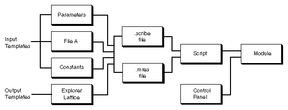
Figure 7-1 Templates and Scripts
Setting Up Templates
Opening a New Template
Figure 7-2 Template Icons
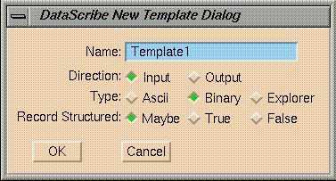
Figure 7-3 New Template Dialog Box
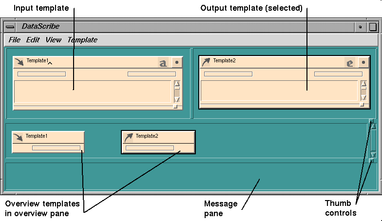
Figure 7-4 Input and Overview Templates
Using the Overview Pane
The Data Type Palette
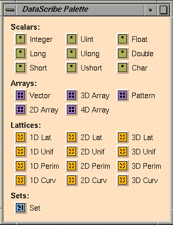
Figure 7-5 DataScribe Data Type Palette
Glyphs
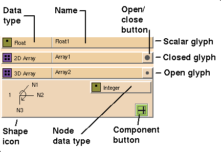
Figure 7-6 Glyph Forms
The Shape Icon
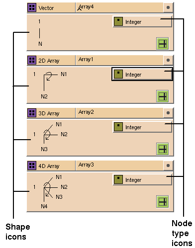
Figure 7-7 The Shape and Node Type Icons
The Node Type Icon
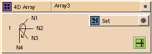
Figure 7-8 A New Array Structure
Figure 7-9 A Hierarchical Array
Component Menu Button
Building a Script
 7  5
90 85 73 57 40 25 14
81 77 66 51 36 23 13
60 57 49 38 27 17  9
36 34 29 23 16 10  6
18 17 14 11  8  5  3
Figure 7-10 An Open Vector Glyph
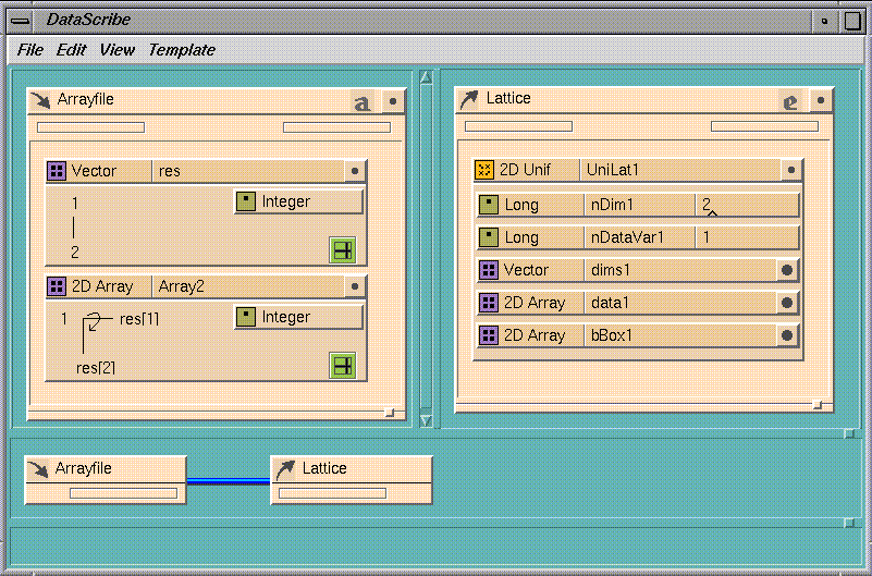
Figure 7-11 A Simple DataScribe Script
Wiring Input and Output Templates
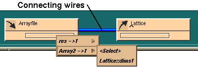
Figure 7-12 Overview Output Port
Running IRIS Explorer
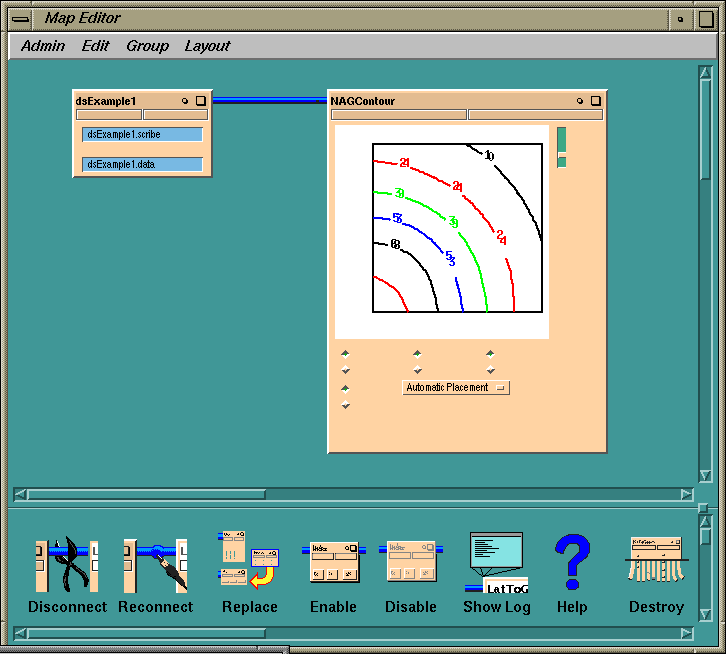
Figure 7-13 The DataScribe Module in the Map Editor
dscribe /usr/explorer/scribe/dsExample1
Designing Templates for Your Data
Reading in Data
Checking EOF
Reading in Lattices
Reading in Binary Files
Data Structures
Category
Elements
Scalars
Char
Short (signed and unsigned)
Integer (signed and unsigned)
Long (signed and unsigned)
Float
DoubleArrays
Vector
2D Array
3D Array
4D Array
PatternsLattices
Uniform lattice (Unif Lat): 1D, 2D and 3D
Perimeter lattice (Perim Lat): 1D, 2D and 3D
Curvilinear lattice (Curvi Lat): 1D, 2D and 3D
Generic input lattice: 1D, 2D and 3DSets
Any collection of scalars, arrays, and/or sets
Scalars
Scalar Glyphs
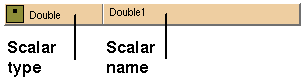
Figure 7-14 A Scalar Glyph
Arrays
Array Glyphs
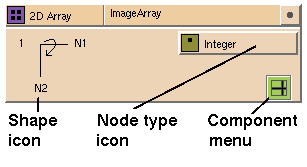
Figure 7-15 An Array Glyph
Hierarchy in Arrays
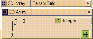
Figure 7-16 A Complex 3D Array
Using Array Indices in Expressions
bBox[1][1]   (Xmin)
bBox[1][2]   (Xmax)
bBox[2][1]   (Ymin)
bBox[2][2]   (Ymax)
Lattices
Lattice Glyphs
Lattice Components
Component
Description
nDim
the number of computational dimensions
dims
a vector indicating the number of nodes in each dimension
nDataVar
the number of data variables per node
primType
the scalar type of the variables (byte, long, short, float, or
double)
coordType
the type of physical mapping:
–
uniform: no explicit coordinates except bounding box coordinates–
perimeter: enough coordinates to specify a non-uniformly spaced rectangular
dataset
–
curvilinear: coordinates stored interleaved at each nodenCoordVar (curvilinear lattices only)
the number of coordinate variables per node
Lattice Types
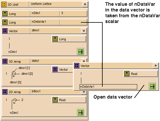
Figure 7-17 A 3D Uniform Lattice
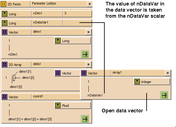
Figure 7-18 A 3D Perimeter Lattice
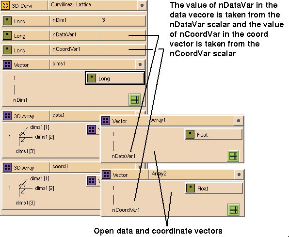
Figure 7-19 A 3D Curvilinear Lattice
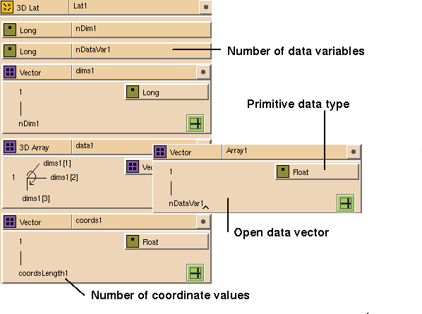
Figure 7-20 A 3D Generic Lattice
Sets
Saving a Set
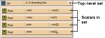
Figure 7-21 A Set for a Bounding Box
Using Nested Sets
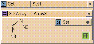
Figure 7-22 Nested Sets
Using a Pattern Glyph
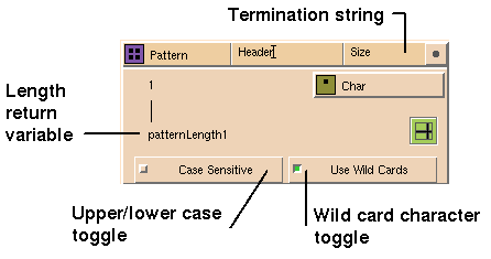
Figure 7-23 A Pattern Glyph
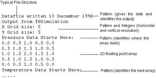
Figure 7-24 File Structure for Pattern Template
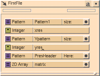
Figure 7-25 An Input Template Using Patterns
Using the Glyph Property Sheet
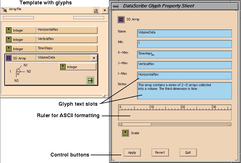
Figure 7-26 The Glyph Property Sheet
Defining Parameters and Constants
Making a Parameters Template
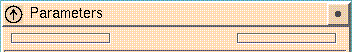
Figure 7-27 Parameters Template Title Bar
Making a Constants Template
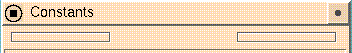
Figure 7-28 Constants Template Title Bar
Connecting Templates
Ordering Variables in a Script
Connecting Data Items Between Templates
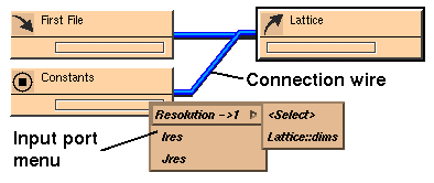
Figure 7-29 Making the First Connection
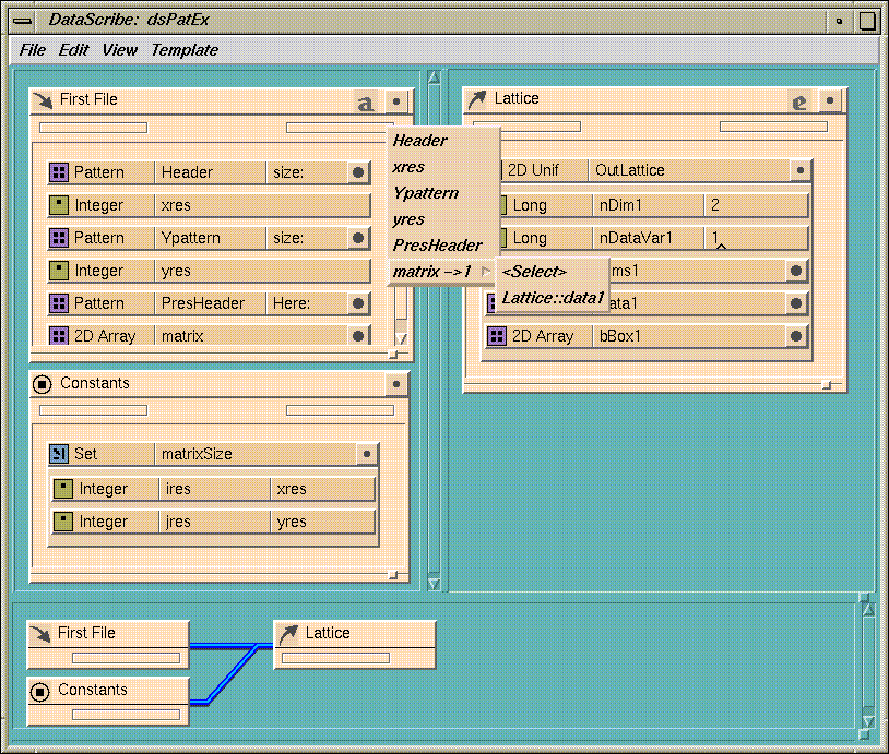
Figure 7-30 A Script Using Patterns
Selecting Array Components
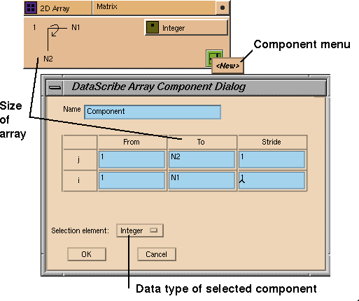
Figure 7-31 Array Component Dialog Window
10                <-- Dimension Variable
10.0 1000.0       <-- Column 1: X Co-ordinate values
20.0 2000.0              Column 2: Data values
30.0 3000.0
40.0 4000.0
50.0 5000.0
60.0 6000.0
70.0 7000.0
80.0 8000.0
90.0 9000.0
100.0 10000.0
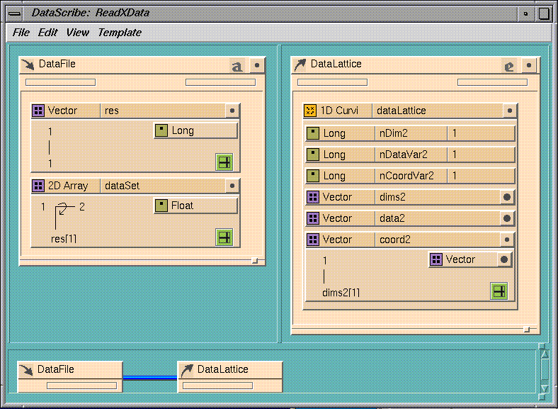
Figure 7-32 Selecting the X Value of a 2D Array
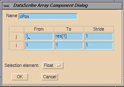
Figure 7-33 Component Dialog Window for X Values

Figure 7-34 Component Dialog Window for Data Values
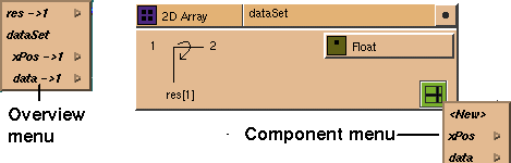
Figure 7-35 New Menus for Input Template
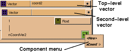
Figure 7-36 Output Lattice Coordinate Vector
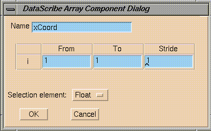
Figure 7-37 Output Coordinate Values (xCoord)
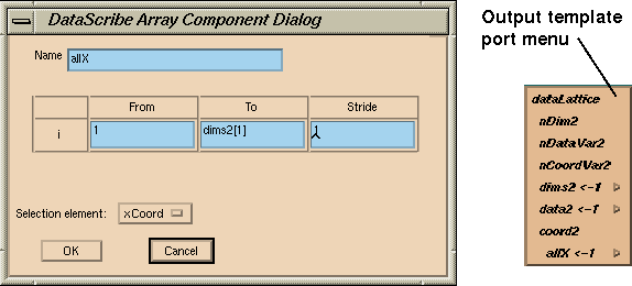
Figure 7-38 Output Coordinate Values (allX)
Converting Formatted ASCII Files
Using the Property Sheet Ruler
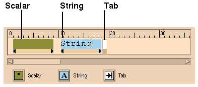
Figure 7-39 The Output Template Ruler
Sample Formatted Data
Resolution is: 8 10 12
Data Follows:
xcoord: 0.000 ycoord: 0.000 zcoord: 0.000 temp: 0.375 pres: -0.375
xcoord: 0.143 ycoord: 0.000 zcoord: 0.000 temp: 0.432 pres: -0.432
xcoord: 0.286 ycoord: 0.000 zcoord: 0.000 temp: 0.403 pres: -0.403
xcoord: 0.429 ycoord: 0.000 zcoord: 0.000 temp: 0.295 pres: -0.295
...
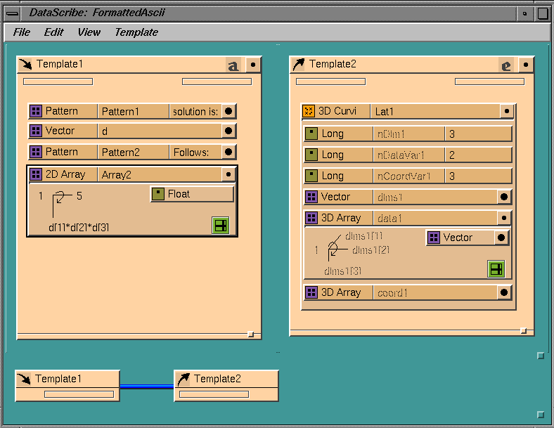
Figure 7-40 Reading a Formatted ASCII File
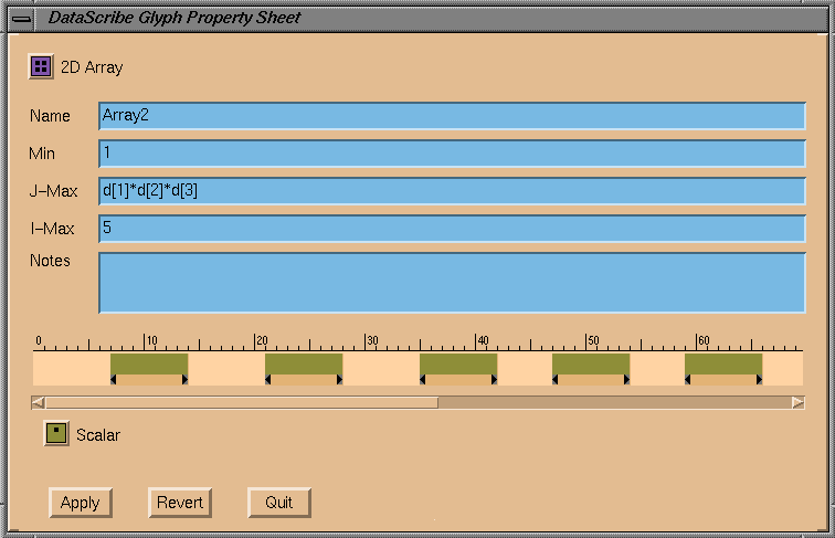
Figure 7-41 Ruler for Reading an ASCII File
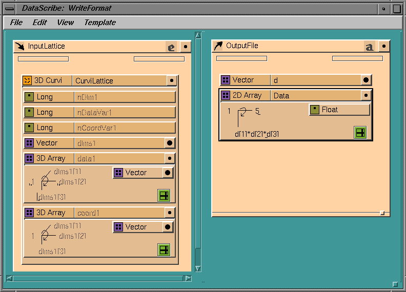
Figure 7-42 Writing a Formatted ASCII File
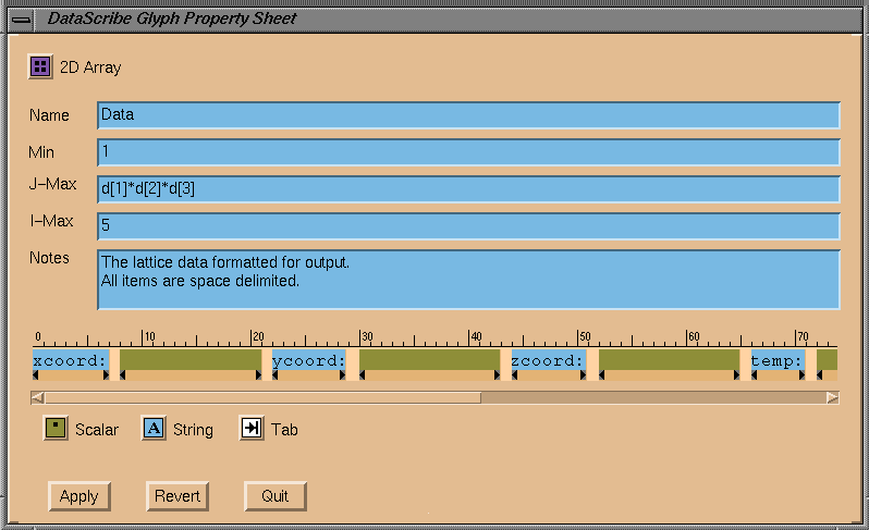
Figure 7-43 An Output Array Ruler
Output from XYZ Simulation
Date: 11 Sept 1991
Resolution 5 10 15
   x-coord	     y-coord     z-coord     function
 0.10000E+01 0.00000E+00 0.00000E+00 0.50000E+00
 0.18000E+01 0.00000E+00 0.00000E+00 0.50000E+00
 0.26000E+01 0.00000E+00 0.00000E+00 0.50000E+00
 0.34000E+01 0.00000E+00 0.00000E+00 0.50000E+00
 0.42000E+01 0.00000E+00 0.00000E+00 0.50000E+00
 0.50000E+01 0.00000E+00 0.00000E+00 0.50000E+00
 0.80902E+00 0.58779E+00 0.00000E+00 0.50000E+00
 0.14562E+01 0.10580E+01 0.00000E+00 0.50000E+00
 0.21034E+01 0.15282E+01 0.00000E+00 0.50000E+00
 0.27507E+01 0.19985E+01 0.00000E+00 0.50000E+00
...
The coordinates and data are interlaced so you need to unravel them by
putting each set of coordinates in the 3D array into a separate output array.
This means collecting
x,
y, and
z
coordinates into three separate arrays using component selection.
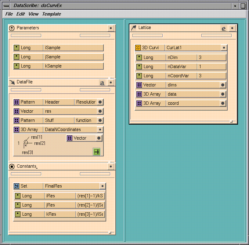
Figure 7-44 A Curvilinear 3D Lattice Reader
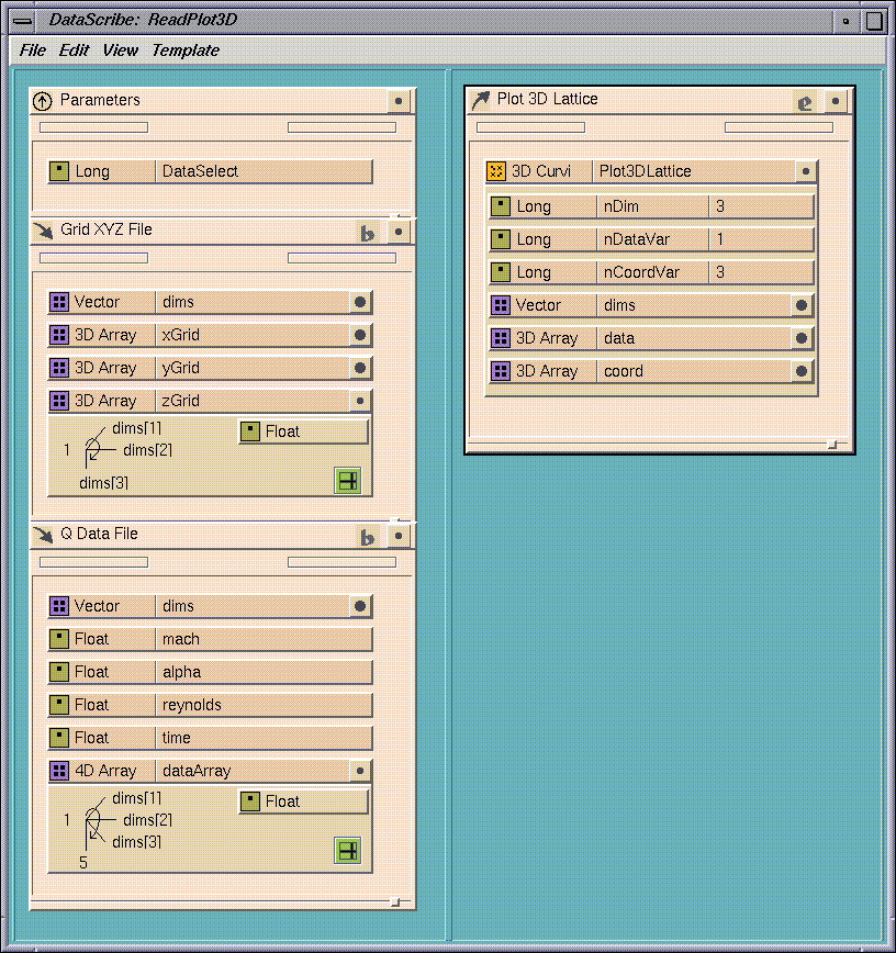
Figure 7-45 The PLOT3D Script
More Complex Expressions
Saving Scripts and Modules
Checking for Errors
Creating a Diagnostic Template
Using a DataScribe Module with the Map Editor
Finding and Correcting Errors
Tracking Down Errors
Interpreting Parsing Messages
Last modified: Mon Oct 13 17:36:59 1997
[ Documentation Home ]