As a language interpreter designed to work with lattices and arrays, the
LatFunction
module runs programs written in Shape and fed to it from
LatFunction's
Program File
or
Program Text
input ports. Shape's syntax is similar to the C programming language. Its
main advantages are that it allows you to work directly with arrays and to
change programs dynamically.
LatFunction
is structured like other modules except that it accepts only lattice and
parameter data. Its ports are wired in the same way as other module ports,
and
LatFunction
makes data on those ports available to the Shape language interpreter as
internal variables. You can:
LatFunction
has two forms. The basic
LatFunction
module has a fixed set of ports, uses fixed variable names for its input and
output data, and does not accept parameters. Working with the second form of
LatFunction,
you create your own module resources to
describe input ports, output ports, and control panel, and you write a Shape
program. The generic
LatFunction
executable then executes in the guise of your module, according to its Shape
program. This is called a
LatFunction-based module. The main differences between the two are the
port names and control panels. Both interpret the Shape language identically.
The
LatFunction
module (see
Figure
10-1) has three input ports, two parameters, and a lattice that controls
its program execution, plus data ports.
You can either enter programs in the
Program Text
input port or load them from a file by typing a filename into the
Program File
file selector.
LatFunction
has fixed names for its data ports. On input, data ports are First In,
Second In, and
Third In. On output, they are
First Out, Second Out, and
Third Out.
A
LatFunction-based module can accept any number of
input parameters and lattices and can output any number of lattices. It does
not output parameters.
The
LatFunction-based module uses the name of an input port, such as
Pressure, to create an internal variable with the same name,
Pressure, in the Shape language. If the input port contains a
non-alphanumeric character (a space is considered a non-alphanumeric
character), the
LatFunction-based module turns that character into an underscore. For
instance, an input port called
Temperature Array
is assigned the internal variable name
Temperature_Array.
A
LatFunction-based module creates internal array variables only for
those input ports that have data. It does not create internal variable names
for ports that do not contain data. This means that you will be able to test
your Shape programs only after all ports that are required for the module
execution have been wired up. The size and shape of the internal array depend
on the port data type, which can be either
parameter
or
lattice.
Parameters on input ports can be of two types:
A scalar, such as the value of a slider widget, is sent to Shape as a
scalar. A character string is sent to Shape as a 1D array of integers
representing the character string in the ASCII collating sequence.
A
LatFunction-based module sends a lattice to Shape in each of three
forms: the data array, the coordinate array, and the combined lattice. The
variable name indicates the form: the suffixes _lat and _coord signify the
combined lattice and the coordinate array, respectively. The variable name
itself signifies the data part of the lattice only. For instance, a
Pressure
port yields data
Pressure, coordinates
Pressure_coord, and lattice
Pressure_lat.
The Shape ports themselves have names derived from the IRIS Explorer
ports. Input ports take the prefix
iport_
followed by the IRIS Explorer port name; output ports use the prefix
oport_. For instance, the port names
iport_Pressure
and
oport_Pressure_Gradient
correspond to the example in
Figure
10-2.
A
LatFunction-based module assumes it must produce data for all of its
output ports. Thus, for each output port name, the
LatFunction-based module uses the internal variable of the same name
to create an output lattice.
Name mapping differs for input and output ports. For input ports, only the
data goes into the variable; for output ports, the variable contains data and
may also contain coordinates.
A
LatFunction-based module distinguishes the different output possibilities
as follows:
Thus,Pressure_lat
can be seen as a list of two arrays, one that contains data and one that
contains location coordinates. If the output array
Pressure_Gradient
has two arrays, they are assumed to be coordinates and data (see
Figure
10-2).
To get coordinates from input to output ports, you must build them into
the Shape internal variable by using
make_lat(coordinates, data). The order of the
arguments is significant: coordinates come first.
For example, suppose a reactor vessel has radially symmetrical pressure
coordinates with pressure data at the nodes. To compute the gradient of the
pressure using
LatFunction, use the following procedure:
Create a gradient program in Shape, using
Pressure
and
Pressure_coord
to compute a gradient field called
Field.
When the
LatFunction
script finishes, the output port contains the pressure gradient based on the
same coordinate system as the input pressure. An output port can use
output_data_flush
to send multiple data sets downstream during one module firing.
The
LatFunction
module takes lattices as its inputs and produces lattices as its outputs, but
Shape operates only on arrays. Shape cannot operate directly on lattices
because each lattice contains two arrays, one for the data and one for its
location coordinates, thus requiring each lattice to be split into its
component parts.
Lattices can have coordinates of three types:
uniform,
curvilinear
and
perimeter, all three of which are acceptable in
Shape. For uniform and curvilinear lattice coordinates, the coordinate array
passed through to Shape consists of the floating point coordinates of the
lattice in whatever type was present on input. This array looks exactly like
the values array of the comparable lattice coordinates structure.
For example, the program to scale an array of data by 3.0 while
maintaining coordinate positions is:
The program to scale a lattice's coordinate positions by 3.0 while
maintaining data values is:
Note: This program works only for uniform and curvilinear
coordinates. Perimeter coordinates are handled separately (see
"List Operators").
You can give your
LatFunction-based module any control panel you want, with any widgets
and any port names. However, every
LatFunction
module must have a widget named "Program File". This widget can be either a
File Browser or a Text Type-in widget but it must deliver a text string. Your
module may also have a radio button widget named "Debug?" This widget
generates debugging printouts when its value is non-zero.
To build a custom LatFunction-based module, follow these steps:
You can now load the module into an IRIS Explorer map.
If you bring up an IRIS Explorer map with a
LatFunction-based module in it, you can now change that module's
execution simply by changing the contents of the program file. Pressing the
Enter
key with the cursor in the "Program File" type-in forces the
LatFunction
module to reread and interpret that file. This, in turn, forces the module to
refire based on a new program.
Note: A refiring caused by the module receiving a different value
from a control panel widget does not cause the program to be
reinterpreted.
Think of a channel selector that takes a three-color RGB (red, green,
blue) image as input. Based on your selection, it sends either red, green, or
blue downstream. You can change the selected channel on a control panel but,
by modifying the program, you can also change the representation of output
data. It is clear that prototyping on the fly has definite advantages when
compared to the more laborious process of creating a module from scratch.
For instance, the following channel selector has three input ports:
and produces one lattice as output:
Its action is to select the red, green, or blue channel of the input data
(Multi_Channels), depending on the value of
Selection, and output a gray-scale image on the output port.
The Selection parameter can be any widget that produces an integer between
0 and 2, inclusive, including a dial, slider, option menu, radio box, or even
a type-in. Values below 0 and above the number of channels of the input are
clipped to the valid range. The program creates a single-channel output. The
shape program
channelselect.shp
and resources file may be found in directory
$EXPLORERHOME/src/MWGcode/LatFunc/Shape. Test the shape program by
connecting the modules:
ReadImg
to
channelselect
to
DisplayImg. Read in the image file
$EXPLORERHOME/data/image/flowers2.rgb
and the shape program
channelselect.shp
and select each of the color channels, 1 to 3, in turn.
Note: Leading // (double slash) characters indicate a Shape comment
line.
The instructions for working with input data are given to
LatFunction
in the form of a Shape program.
As an array-oriented language with a C-like syntax, Shape has many
similarities to C. Shape includes all of C's math library functions (see
Table
10-2), as well as some other common operations. Like C, Shape function
names and variable names are case-sensitive, and Shape has zero-based
indexing. Shape extends the power of C by operating on arrays rather than on
single scalar values.
For instance, if lattice input ports
First In
and
Second In
are of the same size and shape, you can add them to produce a lattice output
port,
First Out, with
Note: Using the
define
operator
:=
is analogous to assigning a pointer to a structure or to an array in C. Here
it makes
First_Out
a reference to the temporary array created by the addition of
First_In
and
Second_In.
Note: This statement creates a lattice
First_Out
which adds the data portions of the lattices
First_In
and
Second_In, and is given default coordinates.
To try this and the next example, wire the output of
GenLat
to ports "First In" and "Second In" of
LatFunction
and wire
LatFunction's "First Out" port to
IsosurfaceLat
and then to
Render.
Multiplication is:
You can compile the array of maximums with the
max
function, a Shape function analogous to the Fortran function
max:
You can produce a double precision output lattice with:
Most other C arithmetic and logical operations work analogously on Shape
arrays. Try:
Shape differs from C in several important ways, including the use of the
define
operator (:=), and the way it manipulates lattices.
In Shape, lattices behave much like arrays in C or Fortran, and they also
resemble arrays in Fortran 90. You can enquire the value of a Shape variable
varname
by inserting the following line in your Shape program:
The examples show the Shape syntax of the computed result with an arrow
symbol (for instance,
==>[[1,2],[3,4],[5,6]]). They also show Shape arrays printed in a
more conventional array layout, such as:
The array
[[[1,2], [3,4]], [[5,6], [7,8]]]
could be displayed equivalently as
For example, in this fragment, the vectors
u,
v, and
r
are declared and allocated, then individual values are assigned as in C.
Finally, the sum of
u
and
v
is copied (with the = operator) to
r.
A Shape array is the same as the data array of an IRIS Explorer lattice.
Its dimensions are identical to those of the IRIS Explorer lattice, with
All
nD lattices in IRIS Explorer are (n+1)D Shape arrays by
default, with the
The
rank
of a lattice is the number of dimensions it has. The
shape
of a lattice is the vector whose entries are the lengths in each dimension.
For example,
[1, 2, 3]
has rank 1 and shape
[3], and
[[1, 2], [3, 4], [5, 6]]
has rank 2 and shape [3, 2]. Rank 1 arrays are often called vectors and rank
2 arrays are often called matrices. An array with rank 0 is a scalar.
Arithmetic with arrays is almost always done element-wise, as follows:
Arrays are automatically promoted to higher rank as required. Promotion
entails augmenting the rank of an array and copying array values to fill in
the new array elements. Lattices promote on the right, in the most rapidly
varying dimension. That is, arrays with the following shapes are compatible
with respect to promotion:
[5, 4, 3], [5, 4], and
[5]. Data values are copied to consecutive array locations during
promotion.
For instance, given
u
from the above example:
Note: As m is a 2D Shape array it is equivalent to a 1D IRIS
Explorer lattice, and you may also view the result of the computation by
wiring up
LatFunction
to
PrintLat:
Note: The fragment above
is not
matrix-vector multiplication
Note: The first line defines m as a 2D Shape array, and assigns
values to it. The second line assigns the Shape vector [1, 2] to m, updating
the values of m.
You can change the direction in which lattices promote: refer to the
Inside,
Outside, and
InsideOut
functions listed under "Miscellaneous" in
Table
10-3
as well as in
"Promotion of Arrays"
and
"Reduction of Arrays".
It is an error to operate on arrays of differing lengths in any dimension.
For example,
[1, 2, 3] + [3, 4]
is an error.
The
define
operator, denoted
var:= value, binds a variable without requiring that the variable be
previously defined.
Define
is not present in C, but it provides functionality similar to that of C
pointers.
The
:=
operator, unlike
=, copies no data. Instead, the value is simply given a new alias,
or name. The
define
operator is important because:
In the first example, a is defined by reference to a part of L, and has no
storage of its own. Allocating the value
5
to a also changes the value of L[1]. In the second example a must be declared
before the value L[1] may be assigned to it. As a is now a separate variable
with its own storage, the value of L[1] is not changed when a is changed.
For example, you could make the statement
The data from the input port may be a whole lattice, and simply labelling
the lattice instead of moving each piece of the lattice to the label is less
work.
Define
is commonly used to change a small part of a lattice. For example, after:
m is now a 5 x 5 identity matrix. In the first line, m is declared to be a
5 x 5 matrix and is initialized with zeros. In the second line, the vector d
is defined as the diagonal of the matrix. Finally, the scalar 1 is promoted
to a vector and added to each entry of d. Since d is an alias for part of m
(the diagonal), the result is that 1 has been added to each entry of the main
diagonal of m.
Arrays promote on assignment and during binary operations. Arrays are
promoted by padding the shape on the right, that is, in the fastest varying
dimension. The promotion iterates each element of the source until the newly
padded dimensions have been filled with the value, then moves on to the next
source value.
Arrays are reduced by compressing the shape on the right, that is, in the
fastest varying dimension. The reduction selects the first element of the
source array in all of the newly reduced dimensions on assignment. On
updating assignment (for example, +=) the dimensions are compressed by the
reduction operator.
Reduction assignment by addition adds the data of the extra dimensions
together. For example:
Assignment reduction looks like a sum over
i
of
inside(A = B[i])
on the correct number of dimensions. The following example shows a few
updating operator reductions:
The
update
operators, such as
+=
and
*=, behave somewhat differently in Shape than in C. For example,
take the expression
x += y.
If
x
has lower rank than
y, then
y
is reduced into
x, as follows:
Note: The fragment above assigns to
x
the sum of the entries of
y.
Reduction occurs along the same dimension as promotion, on the right of
the array's dimension vector.
The base data types in Shape differ from those in C. Shape lacks
char
and all the C-type modifiers, such as
extern, static, unsigned, signed, short,
and
long, but it has the additional data types
byte,
complex
and
double complex.
All the base data types in Shape match the IRIS Explorer data types,
except the two complex types. The complex numbers consist of a pair of
floats, and the double complex numbers consist of a pair of doubles. Complex
numbers must be read into IRIS Explorer as floats or doubles, converted in
Shape, and read out again as floats or doubles.
Table
10-1
compares the data types in the two languages.
Functions are declared differently in Shape than in C. For example, the
C-style declaration
is expressed in Shape as
To summarize:
Table
10-3
lists the built-in functions available in Shape.
Shape's loop syntax is fundamentally identical to that of C. The following
examples illustrate correct usage.
Shape's
for
loop construction is identical to that of C. The three expressions in
parentheses following
for
give the initial setting, test logic, and loop counter changing,
respectively. The code block for the loop can be one statement or a sequence
of statements; if the block is a sequence of statements, it is enclosed in
curly braces. For instance:
Caution: Because the increment operator ++ is not yet implemented,
use the construction i += 1 instead of i++ in loop iterations, as shown
above. Using the ++ operator will produce a "Not Yet" error message.
Shape's
while
loop construction is identical to that of C. The loop iterates while the
conditional expression evaluates to true, or non-zero. For instance, the
for
loop of the previous example could be rewritten as:
Shape's
continue
and
break
statements are identical to those of C. The
continue
statement causes execution in a
for
or
while
loop to branch to the next iteration of the loop. The
break
statement causes execution in a loop to branch out of the loop to the next
higher loop level or to exit from a singly-nested loop.
Shape has the same concept as C of automatic variables, which are freed
when the scope of their declaration is exited. This is useful for memory
allocation, since it relieves you of having to worry about freeing variables.
However, it can be inconvenient at times, particularly when you want to use a
conditional assignment to an array of a variable size. For instance, the
following program fragment is in error:
This Shape program fails to set First_Out because array is freed when its
scope (an if or else clause) is exited. You can circumvent this problem by
creating a function that returns the array, as follows:
Shape offers some features that are not available in C. These include:
See
Table
10-2
and
Table
10-3
for lists of Shape functions.
The
copy
function implements a copy on write (COW) functionality for its single
argument. Its action lies between that of
define
(:=) and
assign
(=) in that it creates a pointer to its argument only if no writes are done
to that pointer. However, when the first write to the returned pointer
occurs, the
copy
function copies the data values of the source. This late binding of copying
is efficient for routines that access input port data; it prevents Shape
programs from writing over input data, but delays making a copy until a
write
is attempted,as shown:
In order not to overwrite the input lattice, b2 rather than b1 should be
used for updating any values related to the input lattice.
Shape's
scatter
and
gather
functions extract data from one array and copy it to another array. The
extracted data need not be arranged in a regular pattern, as is required of
subshape, below. However, the values are copied rather than simply
assigned a pointer, as they would be with
subshape. Thus,
scatter
and
gather
are more expensive than
subshape.
scatter
takes three arguments: the
destination
(dest),
index, and
source
arrays.
scatter's functionality implements the mathematical operation:
which copies each value from source into the dest position specified by
index. Source and dest must have the same type.
The shapes of
index,
source, and
dest
must be such that the last dimension of
index
equals the rank of
dest, and the remaining dimensions of index equal their respective
dimensions in
source. For instance, if source has shape [2,3] and dest has shape
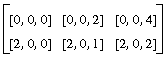
[4,1,6], a valid index would have shape [2,3,3] and might be
[[0,0,0], [0,0,2], [0,0,4]], [[2,0,0], [2,0,1], [2,0,2]]].
With a
source
of
[[1,2,3], [4,5,6]], the resulting
dest
would be
[[[1,x,2,x,3,x]], [[x,x,x,x,x,x]], [[4,5,6,x,x,x]],
[[x,x,x,x,x,x]]].
where x denotes the original value from
dest
before the
scatter
operation was performed.
gather
is a function that returns a gathered array, with two arguments,
index
and
source, interpreted according to the mathematical operation
source(index).
gather
returns the array of selected values in the same shape as index. For example,
with the same
source
array as before, and an
index
[[0,2], [1,1]] the following result is achieved:
The
shape
function returns a dimension vector giving the shape of its input argument.
For instance, a 128 x 256 lattice with three channels of data
(dims = (128,256), nDataVar = 3)
would yield an array of shape
[256,128,3].
The
shape
function is commonly used to discover the rank of an array. An array's rank
is its number of dimensions - essentially, the shape of the shape. The
correct syntax is:
Writing only
would fail, because the returned shape would be a vector of length 1
rather than a scalar rank. The zero-ordered slice extracts the scalar from
its vector position.
The
allocate
function allocates an array of the given shape and type (such as long or
float, as given in the example below) and fills it with values according to
the
fill_type. The basic syntax is:
The fill_type must be one of:
The type of the first argument is used to fix the type of the allocated
array. You may use a known array or value, use a cast value, such as
(byte)1, or use an explicitly typed number, such as
1L
for long or
1.0L
for double.
Slice
extracts a multi-dimensional slice from an array. It has two syntactical
forms. The first one is x[y], where y is a scalar that selects the
yth subarray of
x, exactly as in C. When you use this form, the sliced array has
rank one less than the source. For example, take a 2D array:
Then
a[0] = [1, 2, 3], a three-length vector derived from A in the
ordinary C manner.
The second form of slice is
a[x:y], where
x
and
y
are scalars. In this form an array section, or subarray, of a is extracted.
The subarray has the same rank as a, but contains only slices
x
through
y. For example, given
a, the statement
a[0:1]
extracts two vectors from the original array, and the shape of the array
is [2,
3]. The rank is
2.
In C and Shape, you can write
a[0][0]
to get the first element of a. In Shape, however,
a[0:2][0:1]
is different from
a[0:2,
0:1]. The respective shapes are [2,3] and [3,1], because
a[0:2][0:1]
is the same as
a[0:1].
The
subshape
function takes three or four arguments and returns a reference to a subarray
(or subsection) of its input array. It does not copy any data. The syntax is:
or
where
start, end, and
stride
are vectors of size
shape(source) that signal the indices of the beginning and
end of the array subsection and the strides between successive elements in
each dimension. The default stride is 1. For example, with a 10 x 10
source, you can extract the central 2 x 2 square with
subshape([4,4],[5,5], source) and extract every other row with
subshape([0,0],[10,11],[1,2], source).
An ending index greater than the size of source is legal only if the
actual indices used in the computation do not exceed the array bounds. In
this example, rows 0, 2, 4, 6, 8, 10 would be extracted, but row 11 would
not.
Subshape
does not copy data; it returns a reference to the selected subarray.
The stacking operator concatenates arrays of compatible shape to yield a
new array of rank one higher. The stacking syntax is:
The shape of the stacked array is equal to the shape of the stacked
components, with an added component in the slowest varying dimension. That
component is the number of stacked arrays. For instance, let:
In this case, both a and b have shape
[3], while c has shape
[2,3]. You can change the stacking dimension with
inside.
The
send_indices
function takes an index permutation vector and a lattice. The permutation
controls where each coordinate ends up. As a special case, if permutation
indices agree, then a diagonal is taken in those coordinates. For example:
The 2 x 2 matrix a is transposed because indices 0 and 1 were swapped by
the index vector b.
The new matrix is a diagonal of the 2 x 2 matrix a because the indices
were equal in the index vector b.
Min
and
max
take one or more arguments. With two or more,
min
does an element-wise minimum over all its arguments. With one argument, it
performs a reduction by one coordinate. For example, the first statement
takes the pointwise minimum of three vectors, while the second finds the
minimum element of one vector:
The
dotproduct
operator +.* may be used to form the dot product between vectors and/or
arrays. This is matrix or tensor multiplication.
The form
A+.*B
is identical to the function
dot_product(A,B).
dot_product
has an optional third argument, which directs some number of leading
coordinates
not
to be involved in the product, but, rather, to indicate that several matrix
multiplications of lower rank are to be performed. For instance, if A and B
are
[3,
3,
3]
dimensional arrays, then
dot_product(A, B)
has shape
[3,
3,
3,
3], while
dot_product(A, B, 1) has shape
[3, 3, 3]. The former is a single, 3D tensor product, while the
latter consists of three 2D matrix products.
Bitproduct
resembles
dotproduct, except that it substitutes bit-wise "or" and "and"
functions for addition and multiplication. The
bitproduct
operator is |.&.
The conditional evaluation operator ?: is similar to that of C. When
working with scalar values, its operation is identical to that of C, so
that
evaluates to a if
x
is true (or non-zero) and to b if
x
is false (or zero). The operator goes beyond the C interpretation in that it
can accept arrays as well. In this case, the arrays
x,
a, and
b
must be compatibly shaped. For instance, all three could have the same shape,
or either a or b could be a scalar.
The array operation of
x ? a : b
creates an array the size of x but with values chosen from
a
or
b, depending on the values of
x. Scalars a and b are promoted to constant-filled arrays the shape
of
x, but no additional storage is allocated.
The
inside,
outside
and
insideout
forms are used.
The argument to the inside form is evaluated with different indexing rules
than normal. The four array operations
--
indexing, concatenation (stacking), promotion, and reduction
--
start from the opposite end of the shape vector. For instance,
A[0]
selects the first slice of
A
in the slowest varying dimension, while
inside(A[0])
selects the first slice of
A
in the fastest varying dimension. The former is a
blocked
selection, while the latter is an
interleaved
selection. For example:
The
outside
argument evaluates its argument with the default indexing rules. For example:
The
insideout
argument evaluates its argument with the opposite of the current indexing
rules. Thus,
insideout(inside(expr))
and
outside(expr) are equivalent.
Shape provides some input and output capabilities in addition to creating
array variables from input ports automatically and sending data out on output
ports. For instance, it lets you flush multiple arrays to output lattices
during one computation, and you can also write files.
Before writing a file, you must open it. The file opening commands return
a port identifier as a Shape variable. For instance,
would open an output file.
Note: LatFunction
automatically creates port identifiers, with names such as iport_<portname>
and oport_<portname>, for all the input and output IRIS Explorer
ports on
LatFunction
or a
LatFunction-based module. You can treat
LatFunction
file port identifiers interchangeably with IRIS Explorer port identifiers.
You can write an array
data
to a port identified
by portID
using the
write
command:
If you want this data to enter the IRIS Explorer map immediately, rather
than waiting until module firing finishes, you can use the
flush_output_port
command, as in
In the absence of a flush, the lattice propagates to the map after the
LatFunction
module finishes firing.
You can also write an array to standard output, which can be useful for
debugging, with
Also useful for debugging is the
dump
command, which prints the shape, type, contents, and other information for an
array.
You can write characters on ports with the
write_char
functions, which transmits a single character.
Because IRIS Explorer lattices use their
The function
scalar_lattice_out
adds a trailing unit dimension to an array. It can be used to convert a 2D
Shape array into a 2D IRIS Explorer data array (with nDataVar = 1).
Shape can work with lists of arrays, as well as handle arrays. A list is
an ordered collection of items, each of which can be an array or another
list. For instance, a lattice is represented in Shape as a list of two
arrays:
Note: Lists are delimited by parentheses, not by square
brackets.
The perimeter coordinates of a lattice are stored as individual vectors in
a list. For a three-dimensional lattice, this would be:
Thus the entire lattice would be:
Most Shape commands do not work on lists. Instead, you must either use one
of the special list processing commands or extract an array from the list and
work with it directly. The list processing commands are:
The empty list has its own predefined symbol,
nil.
The
list
function is used to concatenate two or more arrays in
Shape. This can be useful when passing several arguments to a user function,
or when assembling arguments for use in a map or apply call. The syntax for
this function is:
list
uses parentheses
(), not square brackets
[]. It can build arbitrarily complex, heterogenous structures.
list(1,2,3)
is not equal to
[1,2,3]. For example, to create and then concatenate two scalars and
a two-vector:
The two functions
list_first
and
list_rest
decompose lists, extracting the first and all but the first list elements,
respectively. For example:
For perimeter coordinates, the Shape array structure is a list of vectors,
one for each coordinate dimension of the lattice. For instance, 3D data with
perimeter coordinates has three vectors in a list: the first vector
represents the
X
dimension, and the second and third represent the
Y
and
Z
dimensions, respectively.
You can access the list of vectors with the list processing commands,
list_first and
list_rest, which return the first element of a
list and the remainder of the list, respectively. For instance, to access the
X,
Y, and
Z
vectors of a perimeter lattice, you could use:
On output, such a list is interpreted as perimeter coordinates for a
lattice. You can construct a list using the list function and the nil token.
You will need either to write
LatFunction
routines to handle all coordinate types or else restrict inputs to a known
type, using the Module Builder.
The functions
map
and
apply
are used to run a Shape function on a set of inputs. The syntax for these
functions is:
The effects of the calls are different in that
map
runs the named function on each item in the list of inputs, whereas
apply
runs the named function on the concatenated list as a single input:
This is equivalent to concatenating several calls to
sin.
When the list has several arrays in it, the
sin
function works on each input:
This is equivalent to concatenating several calls to
sin.
The
apply
function treats the list as the list of inputs to a single call of the named
function.
This is equivalent to the call:
but is different from the concatenation of calls:
The functions
pair_p
and
null_p
are Boolean predicate functions, each of which indicates the list status of
its argument. Thus,
pair_p
returns
true
(non-zero) if its argument is a list of at least one element (non-empty
list), while null_p returns true if its argument is the empty list of no
elements.
The module prelude is a set of predefined operations that runs when the
LatFunction
module begins firing. They include defining certain mathematical constants,
such as
pi; predefined functions for operations that occur every time the
module fires; and defining useful constants and functional associations.
The postlude is a set of predefined functions that runs when the
LatFunction
module has finished firing. These functions assemble data from known array
names and send it to the output ports. They convert Shape data types back
into IRIS Explorer data types.
These prelude functions run only once, when the
LatFunction
module is first launched. They are:
Predefined Shape functions include.
All
nD lattices in IRIS Explorer are (n+1)D Shape arrays by
default, with the
nDataVar
size taken as the extent of the fastest varying,
n+1, dimension.
These prelude functions run every time the module fires, to organize IRIS
Explorer lattice data into Shape arrays. The example shows prelude functions
for the
LatFunction
ports "First In" and "First Out". Similar operations occur for the other two
ports and for user-defined lattice ports in a
LatFunction-based module.
The postlude functions run as the module completes firing. They convert
Shape arrays back into IRIS Explorer lattice data for each output lattice
port.
The implication of the prelude section is that
First_In,
Second_In, and
Third_In
are Shape variables that contain the input port data for the module. On
output, variables
First_Out,
Second_Out, and
Third_Out
automatically have their data flushed to output ports.
Table
10-2
summarizes the Shape functions that resemble C language functions.
Table
10-3
lists the functions specific to Shape.
Here are three sample programs for the
LatFunction
module.
You can send this program into
VolumeToGeom
and
IsosurfaceLat, which both feed
Render, to get an interesting data set; otherwise, look at the map
testVol. The Shape program may be found in file
$EXPLORERHOME/src/MWGcode/LatFunc/Shape/testVol.shp. Figure
10-3
shows a set of contours displaced from a volume in the Render module. The
program script above produces this volume.
This script allows direct
manipulation of the coloring of an RGB image. It
may be found in
$EXPLORERHOME/src/MWGcode/LatFunc/Shape/ColorXForm.shp
Use the map
ColorXForm.map
in the same directory to view the image. Figure
10-4
shows the results of the color manipulation in the
color-xform
map. The two images shown in
DisplayImg
and
DisplayImg<2>
can be compared.
Use the heat-flux map in the Librarian to view this explicit time-stepping
simulation of a heat flow problem. The
Shape program may be found in
$EXPLORERHOME/src/MWGcode/LatFunc/Shape/Heat_flux.shp. Figure
10-5
shows what the output of the heat-flux program looks like in the
Render
module.
The LatFunction Module
The LatFunction Module
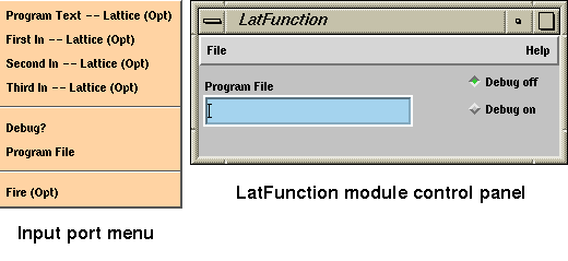
Figure 10-1 The LatFunction Module Control Panel
The LatFunction-based Module
Input Ports
Output Ports
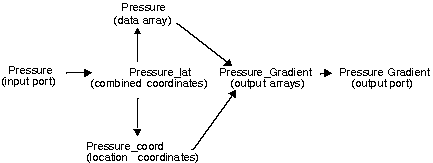
Figure 10-2 How Shape Assigns Variable Names
Pressure_Gradient := make_lat(Pressure_coord, Field);
Interfacing to IRIS Explorer Data Types
First_Out := make_lat(First_In_coord, 3.0* First_In);
First_Out := make_lat(3.0* First_In_coord, First_In);
Building a LatFunction-based Module
Prototyping on the Fly
// Select a specified data channel from the input lattice
// and copy it to the output lattice

// Define sz to be the shape array of the input lattice Multi_Channel
// This is the dimension vector giving the shape of the lattice
// For example [3, 2, 4] for a 3*2 lattice with 4 data values
sz := shape(Multi_Channels);

// Get the rank of the shape array
rank := shape(sz)[0];

// Maximum number of data channels
nChan := sz[rank-1];

// Maximum selectable channels
chan := max(0,min(Selection,nChan-1));

int outsz[rank] = sz;
outsz[rank-1]=1;
Channel_Out := allocate((byte)1, outsz, fill_zero);
Channel_Out = inside(Multi_Channels[chan]);
Shape Language Particulars
Resemblances to C
First_Out:= First_In + Second_In;
First_Out:= First_In * Second_In;
First_Out:= max(First_In, Second_In);
First_Out:= (double) First_In;
First_Out:= sin(First_In);
Differences from C
Lattice Manipulations
write(varname);


int u[3];   int v[3];   int r[3];
u[0] = 1;   u[1] = 5;   u[2] = 10;
v[0] = 2;   v[1] = 3;   v[2] = -3;
r = u + v;
write(r);
==>[3, 8, 7]
u := [1, 2, 3];
v := [4, 5, 6];
write(u * v);
==>[4, 10, 18]
write(u + 2);
==>[3, 4, 5]

m := [[1, 2], [3, 4]];
write(m * [3, 4]);
==>[[3,6],[12,16]]
First_Out := m * [3, 4];
==>[[3,6],[12,16]]

First_Out := m + 1;
==>[[2,3],[4,5]]

m := [[1, 2], [3, 4]];
m = [1, 2];
First_Out := m;
==>[[1,1],[2,2]]

The Define Operator (:=)
L := [1, 2, 3, 4, 5];
a := L[1];
a = 5;
write(L);
==>  [1, 5, 3, 4, 5]
and
int a;
L := [1, 2, 3, 4, 5];
a = L[1];
a = 5;
write(L);
==>  [1, 2, 3, 4, 5]
a:= First_In;
int m[5, 5];       // 5 by 5 array (1D lattice with 5 data variables)
d := diagonal(m);  // point to diagonal of m
d += 1;            // increment the diagonal of m
First_Out := m;    // output lattice
==>  [[1 0 0 0 0],[0 1 0 0 0],[0 0 1 0 0],[0 0 0 1 0],[0 0 0 0 1]]
Promotion of Arrays
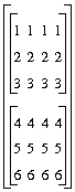
int b[2,3,4];              // declare a 3D array of zeros
a := [[1,2,3],[4,5,6]];    // define a 2D array

b = a;
First_Out = b;
==> [[[1,1,1,1],[2,2,2,2],[3,3,3,3]],
     [[4,4,4,4],[5,5,5,5],[6,6,6,6]]]
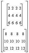
First_Out := b + a;
==> [[[2,2,2,2],[4,4,4,4],[6,6,6,6]],
     [[8,8,8,8],[10,10,10,10],[12,12,12,12]]]
Reduction of Arrays
int b[2, 3, 4];
int c[2, 3];
a := [[1, 2, 3], [4, 5, 6]];
b = a;
c += b;
First_Out := c;
==>  [[4,8,12],[16,20,24]]

// Addition ....
int b[2, 3, 4];
a := [[1, 2, 3], [4, 5, 6]];
long s;
write(s);
==>0
b = a;
s += b;
write(s);
==>84

// Bitwise conjunction of an array ....
s = 1;
write(s);
==>1
s &= b;
write(s);
==>0

s = 1;
write(s);
==>1
s &= [1, 1, 1, 1];
write(s);
==>1

// Logical conjunction of an array ....
s = 1;
write(s);
==>1
s &= (b>0);
write(s);
==>1
Other Operators
int x;
y := [1, 2, 3];
x += y;
write(x);
==>6
int v[3] = 1;
m := [[1, 2], [3, 4], [5, 6]];
v *= m;
write(v);
==>[2, 12, 30]  // the products of each row of m
Data Types
Language
Data Types
C
char, short, int, long, float, double
Shape
byte, short, int, long, float, double, complex, double complex
Function Declaration Syntax
float f(float x, int y) {...; return z;}
function f(x, y) {...; return z;}.
Loop Syntax
For Loop
int i;
double a[5];
for (i=0; i<5; i+=1)
     a[i] = sin(i);            // single statement -- no curly braces
write(a);
==> [0, 0.841471, 0.909297, 0.14112, -0.756802]
While Loop
int i;
int a[5];
i = 0
while (i < 5)
  {
     a[i] = sin(i);
     i += 1;
  }
write(a);
==> [0, 0.841471, 0.909297, 0.14112, -0.756802]
Continue and Break
Issues of Scope
if (n==1)
  {
    array := index_fill([3,1]);
  }
else if (n==2)
  {
    array := index_fill([6,6,2]);
  }
First_Out := array;
function ret_array(n)
{
  if (n==1)
     return index_fill([3,1]);
  else if (n==2)
     return index_fill([6,6,2]);
}

First_Out := ret_array(n);
Additional Features
Copy
a := First_In;       // get the input lattice
write(a);            // assume that a byte lattice has been attached
==> [[200],[171],[73],[107]]

b1 := a[0];          // b1 points to the array element a[0]
b2 := copy(a[0]);    // b2 points to the array element a[0]
                     // but will copy the original value of a[0]
                     // if a[0] is updated
write(b1);
==> [200]
write(b2);
==> [200]

b1 += (byte)3;       // update b1 (assumed to be byte)
write(b1);
==> [203]
write(a);            // this will also update a[0]
==> [[203],[171],[73],[107]]
write(b2);           // b2 will still be equal to the original a[0]
==> [200]
Scatter and Gather
dest(index)= source
index := [[0,2], [1,1]];
source := [[1,2,3], [4,5,6]];
a := gather(index, source);
write(a);
==> [3 5]
Shape
int rank = shape(shape(val))[0];
int rank = shape(shape(val));
Allocate
allocate(base_type_example, shape, fill_type)
a := allocate(1, [3, 1], fill_index);
write(a);
==> [[0],[1],[2]]

a := allocate(1, [3, 3, 2], fill_index);
write(a);
==> [[[0,0],[0,1],[0,2]], [[1,0],[1,1],[1,2]], [[2,0],[2,1],[2,2]]]
Slice
a := [[1,2,3], [2,4,6], [4,8,12], [8,16,24]];
a := [[1,2,3],[2,4,6],[4,8,12],[8,16,24]];
write(a);
==> [[1,2,3],[2,4,6],],[4 8 12],[8 16 24]]

write(a[0]);
==> [1 2 3]

write(a[0:1]);
==> [[1 2 3],[2 4 6]]

write(a[0:2][0:1]);
==> [[1 2 3],[2 4 6]]

write(a[0:2,0:1]);
==> [[1,2,3]]
Subshape
subshape (start, end, source)
subshape (start, end, stride, source)
Stack
[expr, expr, ...]
a:= [1,2,3];
b:= [4,5,6];
c:= [a,b];
==> [[1,2,3],[4,5,6]]
Send_indices
a := [[1,2],[3,4]];
b := [1,0];
write(send_indices(b,a));
==> [[1,3],[2,4]]

a := [[1,2],[3,4]];
b := [1,1];
write(send_indices(b,a));
==> [1,4]

Min and Max
min([1, 2, 3], [4, -2, 6], [7, 8, 9]);
==> [1, -2, 3]

min([1, 2, -2, 3]);
==> -2
DotProduct (+.*)
[1, 2, 3] +.* [4, 5, 0];
==> 14

[[1, 2], [3, 4]] +.* [5, 6];
==> [17, 39]

[5, 6] +.* [[1, 2], [3, 4]];
==> [23, 34]

[[1, 2], [3, 4]] +.*[[5, 9], [10, 13]];
==> [[25 35] [55 79]]

BitProduct (|.&)
Conditional Evaluation (?:)
x ? a : b
Changing Promotion and Reduction Order
Inside
v := [1, 2];
w := [3, 4];
write([v,w]);
==> [[1,2],[3,4]]

write(inside([v, w]));
==> [[1,3],[2,4]]

m := [[1, 2], [3, 4]];
write(inside(m[0]));
==> [1, 3]

v := [0, 0];
write(inside(v += m));
==> [4, 6]

m := [[1, 2], [3, 4]];
write(inside(m + [5, 6]));
==> [[6,8],[8,10]]

Outside
v := [1, 2];
w := [3, 4];
write(outside([v, w]));
==> [[1,2],[3,4]]

m := [[1, 2], [3, 4]];
write(outside(m[0]));
==> [1, 2]

v := [0, 0];
write(outside(v += m));
==> [3, 7]

m := [[1, 2], [3, 4]];
write(outside(m + [5, 6]));
==> [[6 7],[9 10]]

InsideOut
Data Output from Shape
globe := open_output_file ("earthData.rgb");
write(data, portID);
flush_output_port(portID);
write(data);
file:=open_output_file("test.out");
byte a=(byte)65;
write_char(a,file);
==> A (in file "test.out")
Scalar_lattice_in and Scalar_lattice_out
List Operators
(coord, data)
(Xcoord, Ycoord, Zcoord)
((Xcoord, Ycoord, Zcoord), data)
List
list(array [, array] ...)
x := 1;
write(x);
==> 1

y := 2;
write(y);
==> 2

z := [3,4];
write(z);
==> [3,4]

list(x,y,z);
write(list(x,y,z));
==>(1 2 [3 4])
List_first and List_rest
a := (1, 2, 3);
write(list_first(a));
==> 1
write(list_rest(a));
==> (2,3)
Handling Perimeter Lattice Coordinates
X_vector := list_first(Perim_Data_coord);
Y_vector := list_first(list_rest(Perim_Data_coord));
Z_vector := list_first(list_rest(list_rest(Perim_Data_coord)));
Map and Apply
map(func, list...)
apply(func, list...)
map(sin, list(0, 1, 2, 3));
==> (0 0.841471 0.909297 0.14112)
sin(0);
==> 0

sin(1);
==> 0.841471

sin(2);
==> 0.909297

sin(3);
==> 0.14112
map(sin, list([1, 2, 3], [4, 5], [1.1]));
==> ([0.841471, 0.909297, 0.14112], [-0.756802, -0.958924],[0.8912007])
sin([1, 2, 3]);
==> [0.841471 0.909297 0.14112]

sin([4, 5]);
==> [-0.756802 -0.958924]

sin([1.1]);
==> [0.891207]
apply(min, list(3, 4));
==> 3
min(3, 4);
==> 3
min(3);
==> 3

min(4);
==> 4
Pair_p and Null_p
The Module Prelude and Postlude
Prelude Set-up Functions
pi       := 3.14159265358979323844;
e        := 2.71828182845904523536;
i        := make_complex(0, 1);
NaN      := sqrt(-1);
fill_NaN
fill_none
fill_index
fill_zero
function lat_data(lat)
function lat_coord(lat)
function make_lat(coord, data)
function index_fill(s) {allocate(1L, s, fill_index);}
function transpose(m) {send_indices([1, 0], m);}
function diagonal(m) {send_indices([0, 0], m);}
function scalar_lattice_out(x) {inside([x]);}
function scalar_lattice_in(x) {inside(x[0]);}
Prelude Execution Functions
iport_First_In := open_input_lattice("First In");
oport_First_Out := open_output_lattice("First Out");
First_In_lat := read(iport_First_In);
First_In := lat_data(First_In_lat);
First_In_coord := lat_coord(First_In_lat);
Postlude Functions
write(First_Out, oport_First_Out);
Shape Function Tables
Operation
Function Name/Syntax
Notes
Arithmetic
Addition
array + array
Subtraction
array
-
array
Division
array / array
Tensor
Boolean Matrix
Multiplicationarray |.&
array
See
Matrix Multiplication
Matrix Multiplication
array +.* array
Performs a tensor product
Casting
To Byte
(byte)
array
For example,((byte)1.1)
To Short
(short)
array
To Long
(long)
array
To Single Complex
(complex)
array
To Double Complex
(double complex)
array
Integer
Modulo
array % array
Bitwise And
array
&
array
Bitwise Or
array | array
Bitwise Exclusive Or
array ^ array
Left Shift
array
<<
array
Right Shift
array >> array
Logical And
scalar
&&
scalar
Scalar only
Logical Or
scalar || scalar
Scalar only
Logical Not
! array
Preincrement
++ array
Not yet implemented
Postincrement
array ++
Not yet implemented
Predecrement
- -
array
Not yet implemented
Postdecrement
array
- -
Not yet implemented
Relational
Equal To
array == array
Not Equal To
array != array
Greater Than
array > array
Less Than
array
<
array
Greater Than or Equal
array >= array
Less Than or Equal
array
<= array
Complex
Real Part
re(array)
Imaginary Part
im (array)
Make Complex
make_complex
(array, array)
re(make_complex (a, b))
==> a
im(make_complex (a, b))
==> bLanguage Statements
Conditional statement
if(
expr
)
Block
else
else
clause is optional
Block
Block statement;
or
{
statement;
statement;
...}
Function Declaration
function (
array, array, ...)
Block
For Loop
for (
expr; expr; expr)
Block
While Loop
while(
expr)
Block
Define
array := expr
Assign
array = expr
Conditional array value
expr? expr: expr
Evaluates its arguments
completely, unlike the C function
with same syntaxReturn
return
expr;
return;
Continue
continue;
Break
break;
Comment
//
Comment text
Precedes a comment (terminated
by end-of-line) (does not use
/*
as in C)List
(array) or (list, list, ...)
C ordered list of arrays and/or
lists (s-expression)
Math Library
Square Root
sqrt
(array)
Sine
sin
(array)
Cosine
cos
(array)
Tangent
tan
(array)
no complex
Arc Sine
asin
(array)
no complex
Arc Cosine
acos
(array)
no complex
Arc Tangent
atan
(array)
no complex
Hyperbolic Sine
sinh
(array)
Hyperbolic Cosine
cosh
(array)
Hyperbolic Tangent
tanh
(array)
no complex
Exponentiation
exp
(array)
Logarithm
log
(array)
Arc Tangent 2
atan2
(array, array)
no complex
Power
pow
(array)
no complex, also infix(**)
Modulo (floating)
fmod
(array, array)
no complex
Remainder
drem
(array, array)
no complex
Conjugate
conj
(array)
Ceiling
ceil
(array)
no complex
Absolute value
abs
(array)
Truncation
floor
(array)
no complex
Rounding
nint
(array)
no complex:
nint(a)
returns nearest integer roundingSign
sign
(array)
no complex, -1, 0, or 1
Minimum
min
(array, array, ...)
takes 1 or
more argumentsMaximum
max
(array, array, ...)
see Min
Operation
Function Name/Syntax
Notes
Lattice
Copy
copy(array)
Scatter
scatter
(dest array, index array,
source array)
Gather
gather
(index array, source array)
ShapeOf
shape
(array)
Allocate
allocate(base type array, shape
array, fill type
token)
Slice
SubShape
subshape
(start array, end array,
sourcearray)
subshape(start array, end array,
stride array, source
array)
Stack
[expr, expr,
...]
SendIndices
send_indices
(permutation
array, source array)
List Operators
List
list_first
(list)
list_rest(list)First element of a list
List consisting of all but the
first
element of a listMap
map(function, array, ...)
Apply
apply(function, array, ...)
List
list(array, array, ...)
Creates a list
PairP
pair_p(list)
A non-empty list?
NullP
null_p
(list)
An empty list?
Miscellaneous
Inside
inside
(expr)
Outside
outside
(expr)
InsideOut
insideout
(expr)
Port IO
OpenOutputFile
portname
:= open_output_file(filename)
FlushOutputPort
flush_output_port
(portname)
Calls cxOutputDataFlush
Write
write(expr, portname)
Sends ASCII to port
Write
write(expr)
Sends ASCII to standard output
Read
read(portname)
Read from portname
Dump
dump
(array)
Prints array debugging information
WriteChar
write_char
(portname)
Writes a single character
Module Prelude
Constants
pi
3.14
e
2.71
i
make_complex(0,1)
NaN
IEEE constant
Values from
Predefined
Operationsiport_<portname>
iport_First_In
oport_<portname>
oport_First_In
<portname>_lat
First_In_lat full lattice
<portname>_coord
First_In_coord coord part
<portname>
iport_First_In
oport_First_In
First_In data part
nil
List terminator value
Predefined Functions
lat_data(lattice)
Gets data part of lattice
lat_coord
(lattice)
Gets coord part of lattice
make_lat
(lattice)
Data + coord = lattice
index_fill
(shape)
Allocates a long array using
fill_index
transpose
(expr)
Works on a matrix
diagonal
(expr)
Works on a matrix
scalar_lattice_in
(expr)
Removes an inner coordinate of
length 1
scalar_lattice_out
Adds an inner coordinate of
length 1
conform
(expr, expr)
Takes a lattice and a shape and
returns a lattice of the passed
shape, but whose corner has the
values of the passed lattice.
Pads with zero the first output to
Shape.
Sample Programs for LatFunction
To Create a Test Volume
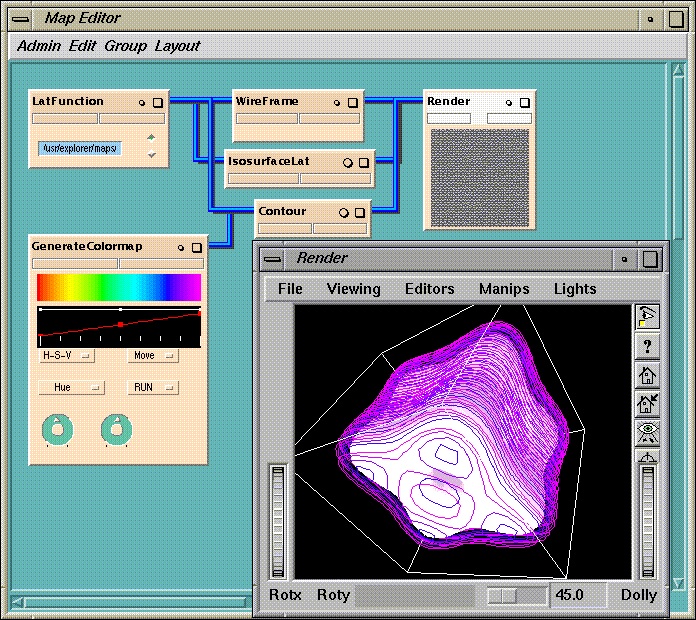
Figure 10-3 LatFunction in the testVol Map
To Carry Out a Color Transform
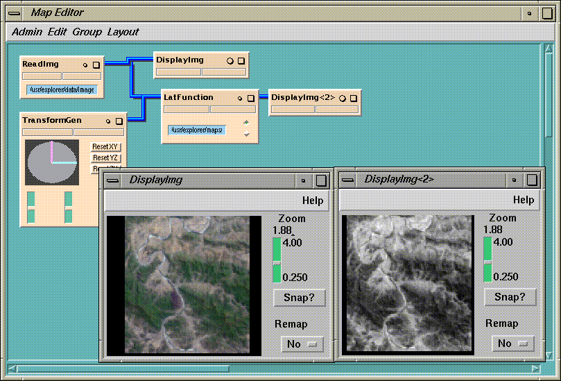
Figure 10-4 Output from the color-xform Map
To Generate a Heat Flux
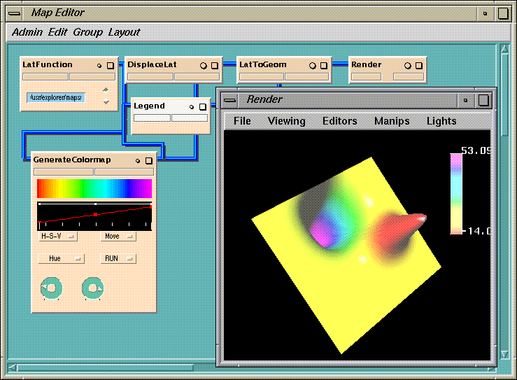
Figure 10-5 Output from the heat-flux Map
[ Documentation Home ]