IBM Visualization Data Explorer QuickStart Guide
[ Bottom of Page | Previous Page | Next
Page | Table of Contents | Partial Table of Contents | Index ]
Partial Table-of-Contents
Importing data into Data Explorer is the first step in creating a visualization
of that data.
Data Explorer supports the importation of a number of data formats:
General Array Importer, Data Explorer native, CDF, netCDF,
and HDF (see Appendix B. "Importing Data: File
Formats" in IBM Visualization Data Explorer User's Guide).
The General Array Importer is discussed here not only because it can
import a variety of data types but because its supporting
interface makes it useful to the broadest range
of users.
This interface consists of the Data Prompter, for describing the data to be
imported, and the Data Browser, for viewing the data.
This chapter deals with the importation of data in the following
sections:
| An Important Note on
Fields |
|---|
|
Importing data into Data Explorer requires some knowledge of the Data Explorer
data
model and at least a working knowledge of a field.
Fields are the fundamental objects in the Data Explorer data model.
A field represents a mapping from some domain to some
data space.
The domain of the mapping is specified by a set of positions
and (generally) a set of connections that allow
interpolation of data values for points between
positions.
Positions represent what can be thought of as (and often really are)
locations in space; the data are the values associated with the
space of the positions.
The mapping at all points in a domain (not just those specified by the
given positions) is represented implicitly by specifying that the
data are dependent on (located at) the sample points or on the
connections between points.
This simple abstraction is sufficient for representing a wide range
of information.
For example, you can describe 3-dimensional volumetric data whose domain
is the region specified by positions and whose data space is the set
of values associated with those positions.
The domain of a 2-dimensional image on a monitor screen is a set of
pixel locations, and the data space consists of the pixel
color.
For 2-dimensional surfaces imbedded in 3-dimensional space (e.g.,
traditional graphical models) the domain may be a set of
positions on the surface, and the data space a set of
data values on that surface.
In Data Explorer the positions and data are said to be components
of a field, and every field must contain at least a
"positions" component and a "data"
component.
Fields may also contain other components (e.g., "connections").
Thus a Data Explorer field consists of data and the additional components
needed to describe that data so that Data Explorer can process it.
(cont.)
|
| An Important Note on Fields
(cont.) |
|---|
|
Components are represented as arrays of numbers with some auxiliary
information specifying attributes (e.g., type of
data dependency).
The syntax of defining fields in the General Array format is described
in 5.3 , "Header File Syntax: Keyword
Statements".
The various components are described in IBM Visualization Data Explorer
User's Guide.
|
To import data through the General Array Importer, you must be able to
answer the following questions.
- What are the independent and dependent variables?
For example, if temperature and wind velocity are measured on a
latitude-longitude grid, then latitude and longitude are
the independent variables, temperature and wind
velocity the dependent variables.
In the case of resistance measurements versus the voltage applied to a
semiconductor, voltage is the independent variable and
resistance the dependent variable.
| Components and Variables |
|---|
|
In Data Explorer terminology, the values of the independent variable constitute
the "positions" component of a data field.
In the examples above, the first independent variable consists of
locations in space and the second does not, but both would be
represented as "positions" in a data field.
The independent variable is always represented by the
"positions" component.
The values of the dependent variable constitute the "data"
component.
|
- What is the dimensionality of the positions and data
components?
In the first example above, latitude and longitude are represented by
2-dimensional positions, the temperature by scalar data, and
the wind velocity by 2- or 3-dimensional vectors.
In the second example, voltage is represented by 1-dimensional
positions and the resistance by scalar data.
- How is the independent variable (the set of positions) to be
described?
By a regular grid (which can be completely described by an origin and
a set of deltas) or by an explicit list (which may or may not
be part of the data file)?
For example, data measurements might be on a grid of 1-degree increments
in latitude and 5-degree increments in longitude;
voltage levels might be a set of unrelated values stored with the
resistances in the data file.
- How are the positions connected to one another, if they are
connected?
For example, a regular grid of positions might be connected by a regular
grid of connections (lines, quads, or cubes).
The connections specify how data values should be interpolated between
positions.
Positions that are explicitly specified (i.e., not regular) can also
be connected by a regular grid of connections (e.g., if the grid
is deformed, or warped).
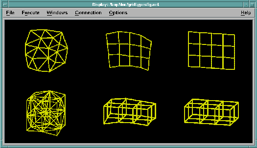
See Figure 11.
Figure 11. Examples
of Grid Types. The three grids in the top row represent surfaces; those
in the bottom row, volumes. Reading from left to right, the three types of grid
are: irregular (irregular positions, irregular connections), deformed regular
(irregular positions, regular connections), and regular (regular positions,
regular connections),

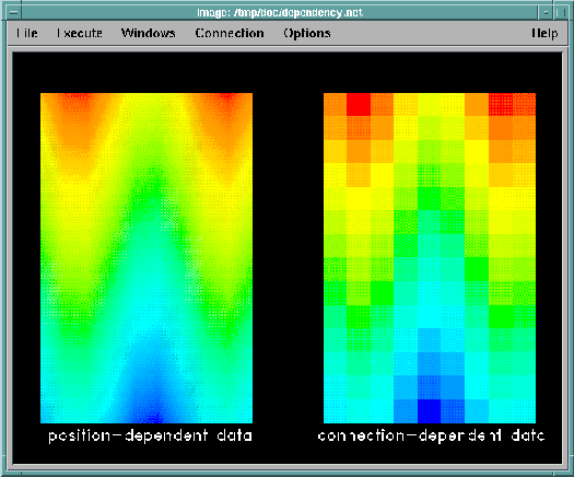
Figure 12. Examples
of Data Dependency. In the visualization on the left, data
correspond one-to-one with positions. Other data values (and colors) are
interpolated linearly between positions. In the visualization on the right, the
elements connecting positions are quads. Data (and colors) correspond one-to-one
with, and are constant within, each quad.

Note: The General Array Importer supports only regular connections
(lines, quads, and cubes) or scattered data.
For irregular connections such as triangles or tetrahedra, you can use
the Data Explorer native format to import your data.
(See IBM Visualization Data Explorer User's Guide.)
- What is the format of the stored data values, ASCII
or binary?
Are they floating point, integer, signed or
unsigned byte, etc.?
- Are the data dependent on "positions" or on
"connections"?
That is, are the data values associated one-to-one with positions or
with the connections between positions? See Figure 12.
(Data associated with connections are often referred to as
"cell-centered.")
With position-dependent data, values between positions are interpolated
within the connection element.
With connection-dependent data, values are assumed to be constant
within the connection element.
- Do these data values represent "series data" or do they
constitute only a single frame of data?
In the example of resistance levels versus voltage, data may exist for each
of a number of different doping levels.
Each doping level could be considered a single data field and the
collection treated as a series.
- Is the data in "record" or "spreadsheet" style?
(See Figure 14.)
- If the data are on a grid, what is the order of the data items with
respect to the grid?
Is it column majority (first index varies fastest) or row majority
(last index varies fastest)?
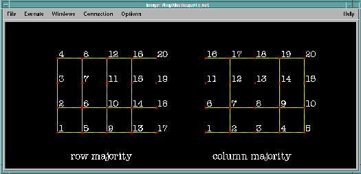
(See Figure 13.)
- What kind of embedded text (comments, etc.) in the data file must
be "skipped" when the data values are read?
With the answers to these questions, you can now use the General Array
Importer to describe your data.
Figure 13. Row-
versus Column-Majority Grids. The two grids shown here are generated
from the same data file, consisting simply of the numbers 1, 2, 3, ..., 20. The
associated header files differ only in the specification of the grids'
majority.

The General Array Importer uses a "header file" to describe the
structure and location of data to be imported.
This file consists of keyword statements that identify
important characteristics of that data (including grid
structure, format, and data type, along with the
path name of the file containing
the data).
A header file can be created with a text editor or, more easily, with
the Data Prompter, which prompts for the necessary information.
(See 3.3 , "Importing Data" for an example
that uses the Data Prompter and
5.4 , "Data Prompter" for a detailed
description of how
to use it.)
The Data Prompter also checks for incorrect syntax, such as conflicting
keywords (see 5.3 , "Header File Syntax:
Keyword Statements").
Once a header file has been created, the data it describes can be
imported into Data Explorer by the Import module.
To identify a header file to Data Explorer through the Import dialog box:
- Enter the path name of the header file in the
name parameter field.
- Enter "general" in the format parameter
field.
(If the file has the extension
".general,"
it is
not necessary to specify the format to Import.
Header files created with the Data Prompter are automatically given this
extension.)
The General Array Importer imports ASCII or binary data that is
organized in one of two general "styles":
block or columnar.
Block
style requires that the data be organized in records,
or blocks.
Columnar
style requires that the data be organized in vertical
columns (see Figure 14).
Figure 14. Block and
Columnar Styles of Data Organization. The three horizontal data blocks
at left illustrate the block style; the three vertical columns at right, the
columnar style. A, B, and C represent separate variables.

The following set of FORTRAN I/O statements generate a record-style
data file:
�write(15,20) A(i),i=1,100
�write(15,20) B(i),i=1,100
�write(15,20) C(i),i=1,100
20 �format(10(f10.3))
An equivalent example in C is shown on the next page.
�for(i=0; i<100, i++) printf("%10.3f",A[i]);
�for(i=0; i<100, i++) printf("%10.3f",B[i]);
�for(i=0; i<100, i++) printf("%10.3f",C[i]);
The following FORTRAN I/O statement produces a columnar-style data
file:
�write(15,10) (A(i),B(i),C(i),i=1,100)
10 �format(3(2x,f10.3))
An equivalent example in C is:
�for (i=0; i<100; i++)
� printf(" %10.3f %10.3f %10.3f\n",A[i],B[i],C[i]);
For both the block and columnar styles, the information in the file
can be positions as well as data.
The data can be:
- scalar or vector
- a time series
- gridded or scattered
(for gridded data the grid structure can be regular or warped, but the
connection elements must be regular; i.e., lines, quads,
or cubes)
- position dependent (associated with the grid positions) or
connection dependent (associated with the grid connections).
[ Top of Page | Previous Page | Next
Page | Table of Contents | Partial Table of Contents | Index ]
[Data Explorer Documentation | QuickStart Guide | User's Guide | User's Reference | Programmer's Reference | Installation and Configuration
Guide ]
[Data Explorer Home
Page | Contact Data
Explorer | Same document on
Data Explorer Home Page ]
[IBM Home Page | Order | Search | Contact IBM | Legal ]
