Reasoning

The concepts used for intelligent control of the pendulum are quite general and can easily be scaled up to more complex systems such as the acrobot.  Also, the code that I generated is also very general and can easily be modified for different systems.  This way the development stage of the project for me, I spent most of my time in this stage of the process.

The technique that I used is a sort of model-based control and minimum time control.  First I developed a model of the system using Mathematica.  Then I wrote a program that used this model of the system to create a look-up table.  I then wrote a non-graphics simulator of the pendulum to test the look-up table.  The next set of programs I wrote had the 332 sending data to the Sun and the Sun was using the look-up table to issue motor commands to the 332.  Finally, I wrote some Matlab code that would re-estimate the model parameters based on collected data.  From these newly re-estimated parameters, I made an improved look-up table.

Here is some Mathematica code fro which you can develop a pendulum inverse dynamics (credits to Chris Atkeson):
Derivation Code

This program used the model of the pendulum to create a look-up table of motor commands indexed by the state of the system (position and velocity).  This look-up table was generated by starting at the goal position and determining the previous states for each of the available motor commands.  Along the way, duplicate and latent trajectories are pruned automatically.

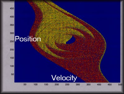
The above picture is a lookup table which stopped when the start state was reached.  The start state is indexed at 250,250 (center of the plot) and the goal state is indexed at 250, 420 (near the top in the middle).  The blue color is either not visited or zero torque command.  The yellow color is a negative torque command.  The red color is a positive torque command.
Table Generator Code (zipped)

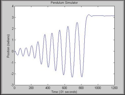
This simulator program simply had the same model of the system that I used to get the look-up table.  For each time step, it used the lookup table just as the real pendulum would.
Simulator Code (zipped)

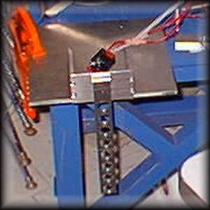
These programs communicated between the 332 and the Sun.  The 332's function was to 1) collect data from the pendulum and send it to the Sun and 2) receive commands from the Sun and translate them into motor commands.  The function of the Sun was to receive data from the 332 about the state of the pendulum, find the appropriate command in the look-up table, and send that command to the 332.
Pendulum Invert Code (zipped)

The Sun program above would not only use the data to get the appropriate motor command, but it would also log the data in files for future use.  Two forms of the data were stored, one that was simply the arguments for the equations of motion and the other was the arguments for the integrated equations of motion.  The following Matlab code uses least squares approximation to return the model parameters.
Parameter Learning Code

There were some problems along the way that were unexpected.  The first was a time lag needed to communicate with the Sun.  The 332 could easily interrupt and issue commands every .01 seconds (or even faster), but the time it took to communicate with the Sun was .03 seconds.  This only makes a difference in 1) the timing of the look-up table since the appropriate delta time value should be used and 2) "catching" the pendulum once it got to the top.

The first problem was easy to fix, the second require more work.  In order to keep the pendulum invert once it was pumped up there, I uploaded a smaller look-up to the 332 itself (since it does not have enough memory to handle the entire look-up table).  The speed of this lookup table (updated motor commands every .01 seconds) was enough to keep the pendulum inverted.  The program below was used to take a small "snapshot" of the inverted region of a larger look-up table.  This table has less gaps than a small table generated from scratch.
Snapshot Code (zipped)

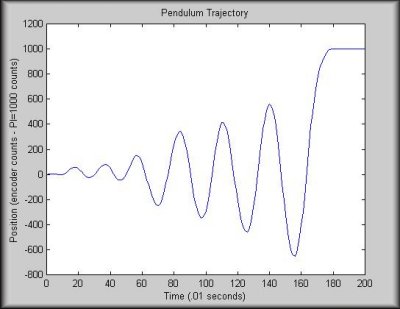
Even in this variation, the pendulum would not always stop on the top.  The look-up table effectively added energy to the system very quickly - the swing-up time was very small, owing to the minimum time control.  However, more often than not, the momentum of the pendulum was enough to swing well past the inverted position instead of stopping.  This could have been a result of not having learned the parameters well enough.  My personal suspicion is that it is a result of the fact that I couldn't use the same look-up table for the entire trajectory and that there are gaps as a result of the switching.

The final problem that I had was that I could never get the two different methods of estimating the model parameters to exactly agree.  One of the parameters would always almost exactly agree, while the other two parameters would be in the same range.  This may have been a result of the discretation of the data, but I could not track down the root of the problem.

In an attempt to solve the discretation problem described above, I tried digital filtering of the data.  I got some filtering to work, but then it started to actually add noise to the system, which was not a good sign, so I moved on when I couldn't track it down.  I have two sets of code here: the Matlab code I used to select filter coefficients (Butterworth digital filter) and the 332/Sun programs that handle the real-time digital filtering.
Matlab Filter Code
Real-time Filter Code (zipped)

Some future work I would have liked to have done if I had more time:
1) fix the problems I described above
2) use a neural network to model the pendulum and use that to generate the look-up table
3) use a neural network to simulate the look-up table
4) convert Gary Boone's simulation code so that it uses a real machine
5) use a DAC to generate a continuous motor torque (rather than bang-bang control)