Project 2: Local Feature Matching
Feature detection and matching are are an essential component of many computer vision applications.In computer vision, features are computing abstractions of image information. Features may be specific structures in the image such as points, edges or objects. Features may also be the result of a general neighborhood operation or feature detection applied to the image. Feature points are used for panorama stiching, image alignment, 3D reconstruction, motion tracking, robot navigation, indexing and database retrieval and object recognition. The goal of this assignment was to create a local feature matching algorithm using techniques described in Szeliski chapter 4.1. The pipeline that I used is a simplified version of the famous SIFT pipeline. The matching pipeline works for instance-level matching -- multiple views of the same physical scene, verified on multiple view images of Notre Dame.
There are three important steps in local feature matching
- Interest Point Detection
- Local Feature Description
- Feature Matching
Interest Point Detection
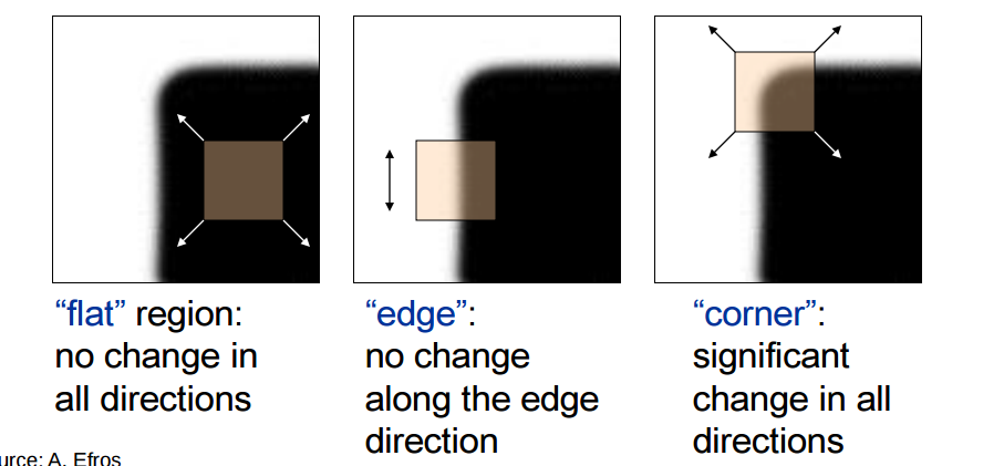
There are many interest point detector algorithms available such as Harris corner point detectors, MSER, Lapacian DOG, etc. In this assignment, I used Harris Corner Point detector algorithm to choose my interest points. Good interest points are distict, repeatable and reproducable. We can recognize corner points by looking for maximum intensity change by moving a small window horizontally and vertcally. As shown in the following diagram, if a point in image is a corner point, then shifting the featire window around that point in all directions will have significant intensity change.
The above chnage in intensity can be calculated using following equation :
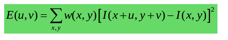
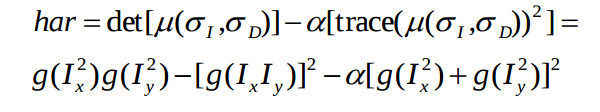
We can apply Taylor series to approximate pars of this equation and to reduce the complexity of corner point calculation. We will get new equatoion as following -
Steps to get interest points :
1) Remove image noise: Apply Gaussian filter (G) over the image, sigma = 0.5
2) Calculate cornerness score (R) Calculate image gradients: Gx, Gy in x and y direction respectively To get Ix, apply Gx on the original image. Calculate the cornerness value for each pixel.
3) Find local maxima: To get good coverage of points across the image and to avoid too many points coming from very small region of the image, I took local maxima using imreginalmax();
4) Now, filter the points on cornerness threshold to get reasonable number of points. I experimented with 3k-20k points. It usually seems to ahve better accuracies when number of points is high.
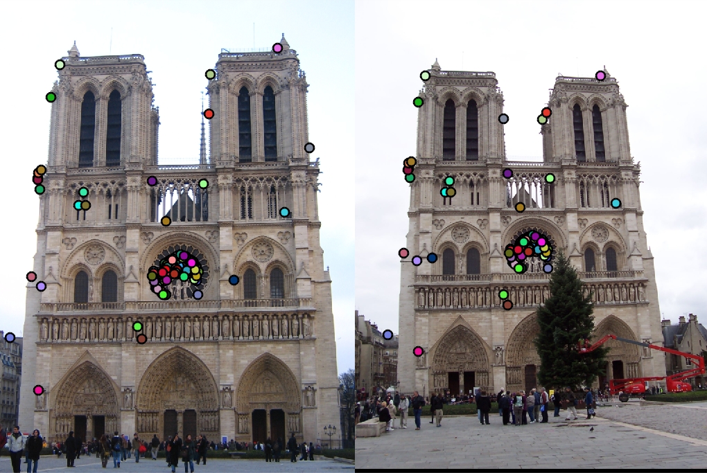
5) Also remove the corner points( not related to cornernes score, but related to pixel location in the image) in the original image. The get_interest_points function retuens a list of x and y co-ordinates of the chosen interest points. Following image shows the chosen interest points in two views of Notre Dame sample images :
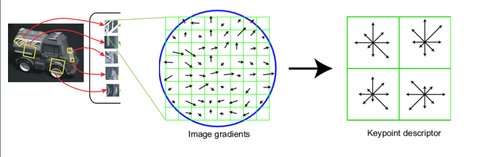
Local Feature Description
Used SIFT feature matching algorithm. For each of the interest points, consider feature_width* feature_width window around it and create a 1* (feature_width*feature_width) feature vector.
SIFT is computed on rotated and scaled version of window according to computed orientation & scale.
Steps in creating SIFT vectors :
1. Smoothened the image and get its gradient magnitude and orientation.
2. Divide feature window( Default: 16*16) around each of interest point in 4*4 cells.
3. Get histogram count of the cell in 8 directions in each cell. You will get output of 1*16 from each cell. Concat outputs of 16 cells and for each point, you will get 128 features.
4. Normalize the feature values and clamp the high value features to some ceratin value (0.2). This will help to avoid high contributio of only some directions in overall cell feature values
Feature Matching
Once you ahve independently found interest points in two images and have created respective feature vectors, these featre vectors from two images can be compared to find the matching vectors and hence, points. Used NNDS ( Nearest neighbour distance ratio) for matching features. Steps :1. For each 128-dimensional feature vector in image 1, calculate its Euclidean distance to each of other point in image 2. ( Used matlab function pdist2())
2. Find two nearest neighbors, min1, min2.
3. Calculate confidence = min2/min1 for each point.
4. Choose top 100 matching point pairs with max confidence.
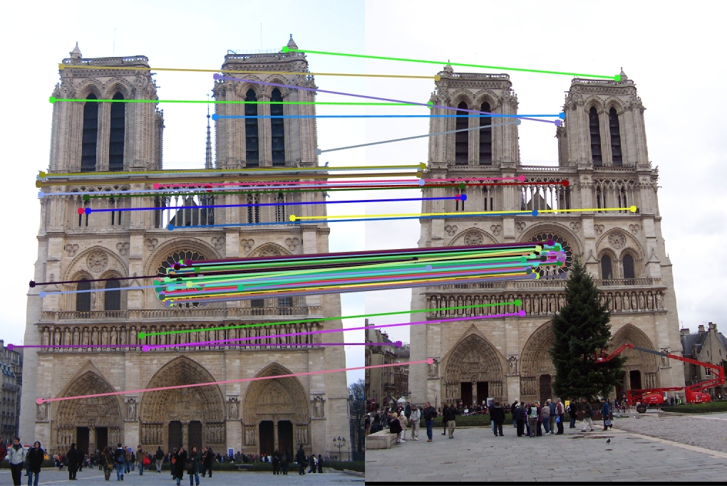
Matched points in Notre Dame.
Evaluation
The matched points' pairs were evaluated against known ground truth for the given images. And 94% accuracy was achieved when ~3k points were chosen in get_interest_points.
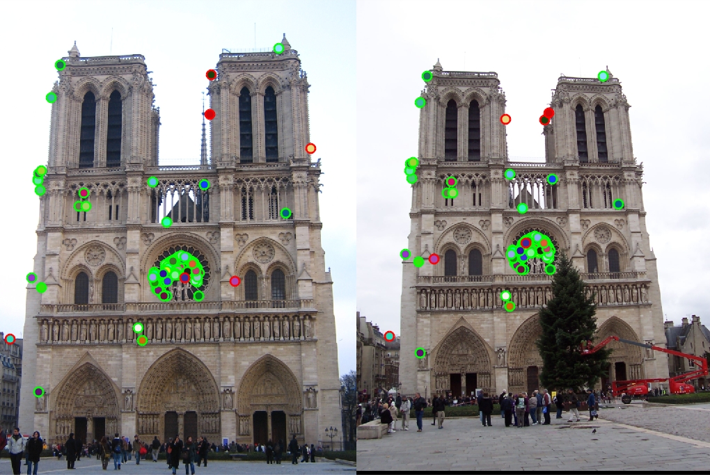
Notre Dame: 94% accuracy
Other Examples of Local Feature Matching
Munt Rushmore 43% accuracy.
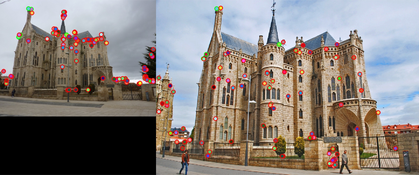
Episcopal Gaudi 5% accuracy.
It was observed that tuning of following parameters was important to get good accuracy - 1) Gaussian filter sigma and size for smoothening the image 2) Corenerness Threshold value above which you would choose the given point as your interest points. 3) Confidence threshold/ nuber of matching pairs chosen for evaluation.
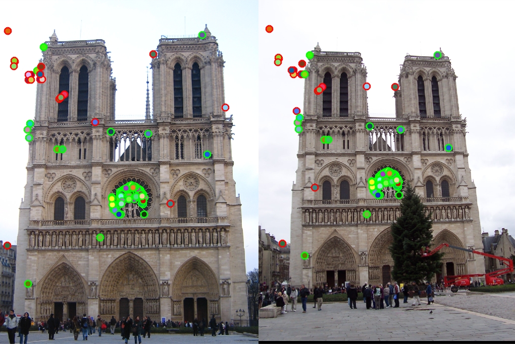
Extra Credits :
1. Chose interest points at multiple scales - 1 (original), 0.5, 0.25, 0.125 2. Chose feature points on multiple scales - 1, 0.5, 0.25, 0.125 Accuracy achieved on Notre Dame (w/ threshold tuning) = 80%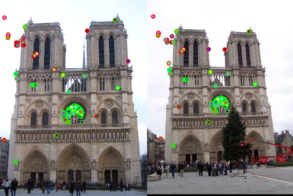
Scale invarinat get_interest_points and get_features : 80% accuracy.