Project 4 / Scene Recognition with Bag of Words
|
The following writeup is organized as follows:
I. Tiny Images with K-nearest neighbors
II. Tiny Images with Linear SVM Classifier
III. Bag of Sift features with K-nearest neighbors
IV. Bag of Sift features with Linear SVM classifier
V. Bag of Spatial Sift features with K-nearest neighbors
VI. Bag of Spatial Sift features with Linear SVM classifier
VII. Bag of Soft Spatial Sift features with K-nearest neighbors
VIII. Bag of Soft Spatial Sift features with Linear SVM classifier
IX. GIST features with K-nearest neighbors
X. GIST features with Linear SVM classifier
XI. GIST + Bag of Soft Spatial Sift features with K-nearest neighbors
XII. GIST+Bag of Soft Spatial Sift features with Linear SVM classifier
- Tiny Images with K-nearest neighbors
- Tiny Images with Linear SVM Classifier
- Bag of Sift features with K-nearest neighbors
- Bag of Sift features with Linear SVM classifier
- Bag of Spatial Sift features with K-nearest neighbors
- Bag of Spatial Sift features with Linear SVM classifier
- Bag of Soft Spatial Sift features with K-nearest neighbors
- Bag of Soft Spatial Sift features with Linear SVM classifier
- GIST features with K-nearest neighbors
- GIST features with Linear SVM classifier
- GIST + Bag of Soft Spatial Sift features with K-nearest neighbors
- GIST+Bag of Soft Spatial Sift features with Linear SVM classifier
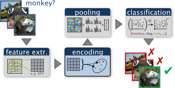
I have used the following algorithm for scene recognition using tiny image representation as features and k-nearest neighbors for classification.
1. Resize each image to a fixed resolution (used 16x16 here) and construct a feature vector by using just the intensity values at each pixel. Obtain such features for each image in the training dataset.
2. For each test image, obtain the feature of the image as described above and used K-nearest neighbors and assign the majority label among the K-nearest neighbors found using the euclidean distance metric. (used k=1)
I have calculated the accuracy and the confusion matrix using 16x16 as the resolution and value of the parameter K=1 in K-nearest neighbors.
It runs under 10minutes.
Following are the results using this parameters.
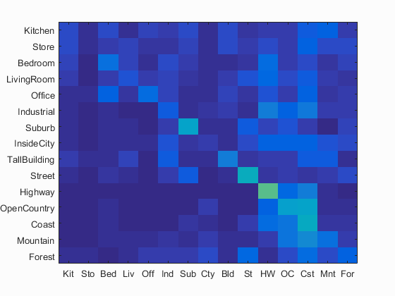
Accuracy (mean of diagonal of confusion matrix) is 0.224 with resolution 16x16 and K=1 in K-nearest neighbors
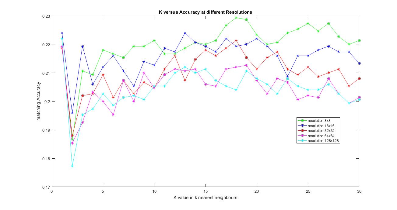
Following is an analysis of the various parameters involved in this pipeline. I have tried varying the resolution size from 8x8, 16x16, 32x32, 64x64 and 128x128 and values of K from 1 to 30.
Observations:
1. As I increased the resolution size, the time taken for obtaining features has increased significantly, but there was not much improvement in accuracy (it decreased the accuracy as you can see from the plot).
2. As I increased the value of K, there was no significant improvement in performance either but the time taken to compute the predicted label for each image has increased.
The image below shows the results of accuracy versus the values of K varying from 1 to 30 and the resolution size from 8x8, 16x16, 32x32, 64x64 and 128x128.
|
The best possible accuracy achieved with this method was 22.9% with resolution 8x8 and K=18 in K-nearest neighbors
I have used the following algorithm for scene recognition using tiny image representation as features and Linear SVM model for classification.
1. Resize each image to a fixed resolution (used 16x16 here) and construct a feature vector by using just the intensity values at each pixel. Obtain such features for each image in the training dataset.
2. Using the training data, train a 1-vs-all linearSVMs for each category which will be later used while testing.
3. For each test image, obtain the features of the images as described above and used 1-vs-all linear SVMs for each category separately and choose the label with maximum confidence. ( used lambda = 10 for better performance)
I have calculated the accuracy and the confusion matrix using 16x16 as the resolution and value of the parameter lambda=10 since I found better performance using this value in SVMs.
It runs under 10minutes.
Following are the results using this parameters.
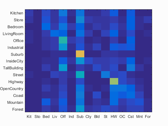
Accuracy (mean of diagonal of confusion matrix) is 0.21 with resolution 16x16 and lambda =10 in 1-vs-all linear SVM
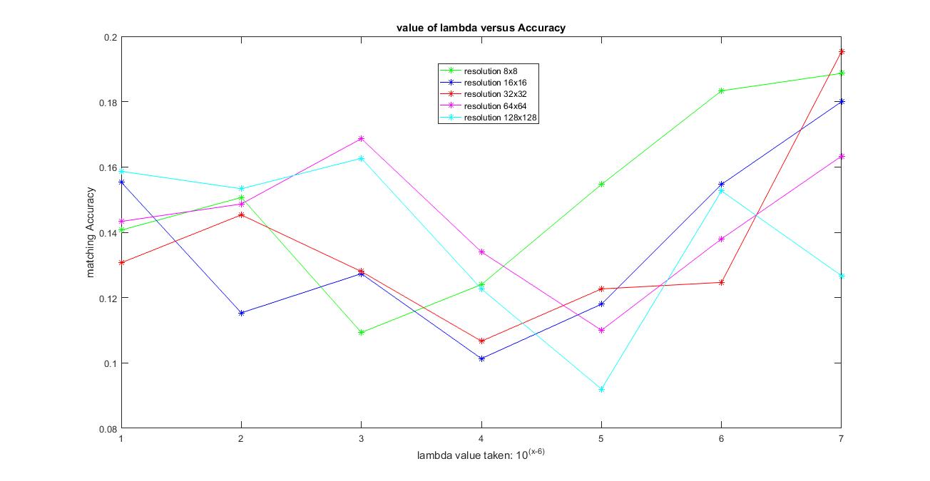
Following is an analysis of the various parameters involved in this pipeline. I have tried varying the resolution size from 8x8, 16x16, 32x32, 64x64 and 128x128 and values of lambda varying from 0.00001, 0.0001, 0.001, 0.01, 0.1, 1 and 10.
Observations:
1. As I increased the resolution size, the time taken for obtaining features has increased significantly, I found certain cases where the performance has improved as you can see from the plot below.
2. As I increased the value of lambda value, the time taken has reduced to compute the predicted label for each image and the performance improved in a few cases and dropped in a few. There was no clear pattern observed.
The image below shows the results of accuracy versus the values of lambda varying from 0.00001, 0.0001, 0.001, 0.01, 0.1, 1 and 10 and the resolution size from 8x8, 16x16, 32x32, 64x64 and 128x128.
|
The best possible accuracy achieved with this method was around 22% with resolution 32x32 and lambda =10 in 1-vs-all linear SVM
I have used the following algorithm for scene recognition using Bag of Sift features and k-nearest neighbors for classification.
1. Extract SIFT features for each training image (used parameter values: step equal to 8 and size equal to 16, fast). Using all the SIFT features (used all samples here) for each image and construct a vocabulary of vocab_size (used vocab_size = 500) using kmeans. This is a one-time operation and the vocabulary is saved then for later runs.
2. Extract SIFT features for each training and testing image (used paramaters: step equal to 4, size equal to 16,fast) and then construct Histogram of SIFT features by maintaining a count into which cluster center each SIFT feature in the image is closest to. Construct this histogram by using a sample of features obtained from that particular image(here sampled about 500 sift features and used them in constructing the histogram of that particular image).
3. Obtain such histogram for each training and testing image and now these are to used as Features for the next steps.
4. For each test image, obtain the feature of the image as described above and used K-nearest neighbors and assign the majority label among the K-nearest neighbors found using the euclidean distance metric. (used K=8)
I have calculated the accuracy and the confusion matrix using the bag of sift features model and the values of the paramaters used: step equal to 4, size equal to 16,'fast' for get_bags_of_sifts using a vocabulary of size 500 and sampling about 500 feature vectors for the construction of the histogram. The value of the parameter K=8 in K-nearest neighbors.
It runs under 10minutes.
Following are the results using this parameters.
Accuracy (mean of diagonal of confusion matrix) is 0.547 with the values of the paramaters used: step equal to 4, size equal to 16,'fast' for get_bags_of_sifts using a vocabulary of size 500 and sampling about 500 feature vectors for the construction of the histogram. The value of the parameter K=8 in K-nearest neighbors.
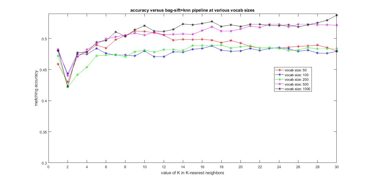
Following is an analysis of the various parameters involved in this pipeline. I have tried varying the vocabulary size from 50,100, 200, 500 and 1000. I have always used the same paramters for the sift features: step-4,size-16,'fast'. I used all the features from the training and testing images to construct their histogram which is used as features and the value of K varying from 1 to 30 in k-nearest neighbors.
Observations:
1. As I increased the vocabulary size, although the time taken is increasing slightly, the accuracy is also improving as you can see from the plot below.
2. As I increased the value of K in k-nearest neighbors, the time taken has reduced to compute the predicted label for each image and there was not much of improvement in performance although it did help in a few cases.
The image below shows the results of accuracy versus the vocabulary size from 50,100, 200, 500 and 1000 and using all the features from the training and testing images to construct their histogram which is used as features and the value of K varying from 1 to 30 in k-nearest neighbors.
|
The best possible accuracy with this Bag-of-features+KNN pipeline achieved was around 54.9% using vocab_size=1000 and k=30
I have used the following algorithm for scene recognition using Bag of Sift features and k-nearest neighbors for classification.
1. Extract SIFT features for each training image (used parameter values: step equal to 8 and size equal to 16,fast). Using all the SIFT features (used all the samples here) for each image and construct a vocabulary of vocab_size (used vocab_size = 200) using kmeans. This is a one-time operation and the vocabulary is saved then for later runs.
2. Extract SIFT features for each training and testing image (used paramaters: step equal to 4, size equal to 16, fast) and then construct Histogram of SIFT features by maintaining a count into which cluster center each SIFT feature in the image is closest to. Construct this histogram by using a sample of features obtained from that particular image(here sampled about 500 sift features and used them in constructing the histogram of that particular image).
3. Obtain such histogram for each training and testing image and now these are to used as Features for the next steps.
4. Using the features of the training data, train a 1-vs-all linearSVMs for each category which will be later used while testing. (used lambda=1)
5. For each test image, obtain the features of the images as described above and used 1-vs-all linear SVMs for each category separately and choose the label with maximum confidence.
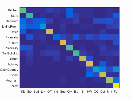
I have calculated the accuracy and the confusion matrix using the bag of sift features model and the values of the paramaters used: step equal to 4, size equal to 16, fast for get_bags_of_sifts using a vocabulary of size 500 and sampling about 500 features for each image for construction of histogram. The value of the parameter lambda = 1 in Linear SVM.
It runs under 10minutes.
Following are the results using this parameters.
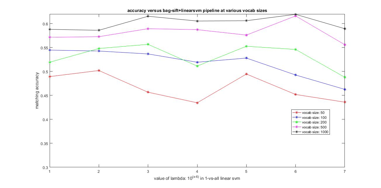
Accuracy (mean of diagonal of confusion matrix) is 0.591 with the values of the paramaters used: step equal to 4, size equal to 16, fast for get_bags_of_sifts using a vocabulary of size 500 and sampling about 500 features for each image for construction of histogram. The value of the parameter lambda = 1 in Linear SVM.
Following is an analysis of the various parameters involved in this pipeline. I have tried varying the vocabulary size from 50,100, 200, 500 and 1000. I have always used the same paramters for the sift features: step-4,size-16,'fast'. I used all the features from the training and testing images to construct their histogram which is used as features values of lambda in SVM varying from 0.00001, 0.0001, 0.001, 0.01, 0.1, 1 and 10.
Observations:
1. As I increased the vocabulary size, although the time taken is increasing slightly, the accuracy is also improving as you can see from the plot below.
2. As I increased the value of lambda value, the time taken has reduced to compute the predicted label for each image and the performance improved in a few cases and dropped in a few. There was no clear pattern observed.
The image below shows the results of accuracy versus the vocabulary size from 50,100, 200, 500 and 1000 and using all the features from the training and testing images to construct their histogram which is used as features and the value of of lambda varying from 0.00001, 0.0001, 0.001, 0.01, 0.1, 1 and 10 in linear SVM.
|
The best possible accuracy using the Bag-of-sift+LinearSVM pipeline achieved was around 62.5% using vocab_size=1000 and lambda = 1 in linear SVM
I have used the following algorithm for scene recognition using Bag of Spatial Sift features and k-nearest neighbors for classification.
1. Extract SIFT features for each training image (used parameter values: step equal to 4 and size equal to 16, fast). Using all the SIFT features (used all the samples here) for each image and construct a vocabulary of vocab_size using kmeans. This is a one-time operation and the vocabulary is saved then for later runs.
2. Extract SIFT features for each training and testing image (used paramaters: step equal to 4, size equal to 16,fast) and then construct Histogram of SIFT features by maintaining a count into which cluster center each SIFT feature in the image is closest to. Construct this histogram by using a sample of features obtained from that particular image(here sampled all the feature vectors from each image for constructing the histogram of that particular image for good performance).
3. level-1: Now repeat the step2 by dividing the image into 2x2 and extract histograms for each sub-part of the image, so we will obtain 4 additional histograms now.
4. level-2: Now again repeat step2 by dividing the original image into 4x4 and extract hostograms for each of these sub-parts. We will have 16 histograms at this level.
5. two ways to implement this, level-1: use level-0 and level-1 features: concatenate them and use them as features
(or) level-2: use level-0, level-1 and level-2 features: concatenate them and then use them as features.
6. Obtain such histogram for each training and testing image and now these are to used as Features for the next steps.
7. For each test image, obtain the feature of the image as described above and used K-nearest neighbors and assign the majority label among the K-nearest neighbors found using the euclidean distance metric.
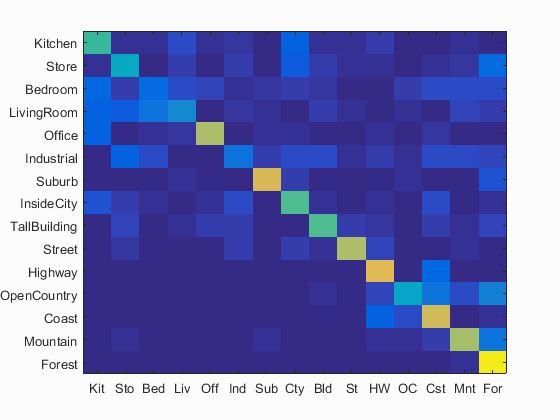
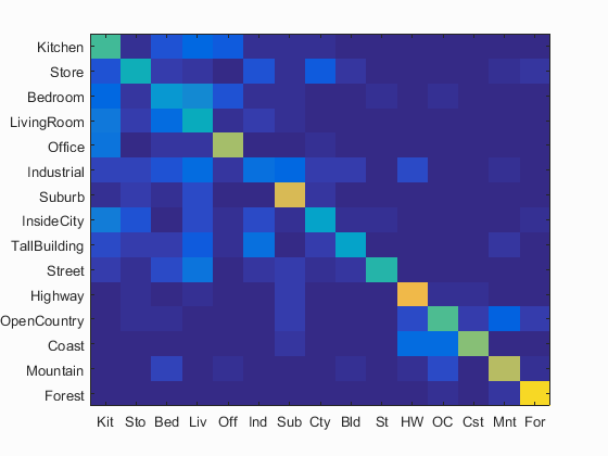
I have calculated the accuracy and the confusion matrix using the bags_sift_spatial_features model and the values of the paramaters used: step equal to 4, size equal to 16,fast and sampled all features,used level=2 for get_bags_of_sifts using a vocabulary of size 500 and value of the parameter K=25 in K-nearest neighbors. Following are the results using this parameters.
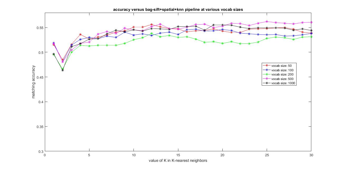
Accuracy (mean of diagonal of confusion matrix) is 0.561 with the values of the paramaters used: step equal to 4, size equal to 16,fast and sampled all features, used level=2, for get_spatial_bags_of_sifts using a vocabulary of size 500 and value of the parameter K=25 in K-nearest neighbors.
Following is an analysis of the various parameters involved in this pipeline. I have tried varying the vocabulary size from 50,100, 200, 500 and 1000. I have always used the same paramters for the sift features: step-4,size-16,'fast',level=2. I used all the features from the training and testing images to construct their histogram which is used as features and the value of K varying from 1 to 30 in k-nearest neighbors.
Observations:
1. As I increased the vocabulary size, the time taken is increasing slightly but here there was no clear improvement of performance as you can see from the plot below.
2. As I increased the value of K in k-nearest neighbors, the time taken has reduced to compute the predicted label for each image and there was not much of improvement in performance although it did help in a few cases.
The image below shows the results of accuracy versus the vocabulary size from 50,100, 200, 500 and 1000 and using all the features from the training and testing images to construct their histogram which is used as features and the value of K varying from 1 to 30 in k-nearest neighbors.
|
Clearly, adding spatial information by using level-2 Spatial-Bag-of-Sift+KNN has improved the accuracy compared to the plain Bag-of-Sift+KNN pipeline. The best possible accuracy with this Spatial-Bag-of-features+KNN pipeline achieved was around 56.1% using vocab_size=500 and k=25
I have also calculated the accuracy and the confusion matrix using the bags_sift_spatial_features model and the values of the paramaters used: step equal to 4, size equal to 16,fast and sampled all features,used level=1 for get_bags_of_sifts using a vocabulary of size 500 and value of the parameter K=11 in K-nearest neighbors. Following are the results using this parameters.
Accuracy (mean of diagonal of confusion matrix) is 0.549 with the values of the paramaters used: step equal to 4, size equal to 16,fast and sampled all features, used level=1, for get_spatial_bags_of_sifts using a vocabulary of size 500 and value of the parameter K=11 in K-nearest neighbors.
I have used the following algorithm for scene recognition using Bag of Spatial Sift and svm for classification.
1. Extract SIFT features for each training image (used parameter values: step equal to 8 and size equal to 16,fast). Using all the SIFT features (used all the samples here) for each image and construct a vocabulary of vocab_size using kmeans. This is a one-time operation and the vocabulary is saved then for later runs.
2. Extract SIFT features for each training and testing image (used paramaters: step equal to 4, size equal to 16, fast) and then construct Histogram of SIFT features by maintaining a count into which cluster center each SIFT feature in the image is closest to. Construct this histogram by using a sample of features obtained from that particular image(here used all of the feature vectors from each image for constructing the histogram of that particular image for better performance).
3. Obtain such histogram for each training and testing image and now these are to used as Features for the next steps.
4. Using the features of the training data, train a 1-vs-all linearSVMs for each category which will be later used while testing.
5. For each test image, obtain the features of the images as described above and used 1-vs-all linear SVMs for each category separately and choose the label with maximum confidence.
I have calculated the accuracy and the confusion matrix using the bags_sift_spatial_features model and the values of the paramaters used: step equal to 4, size equal to 16,fast, sampled all the features and level=2, for get_spatial_bags_of_sifts using a vocabulary of size 1000 and value of the parameter lambda = 0.1 in Linear SVM. Following are the results using this parameters.
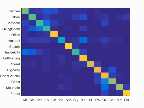
Accuracy (mean of diagonal of confusion matrix) is 0.681 with the values of the paramaters used: step equal to 4, size equal to 16,fast, sampled all the features and level=2, for get_spatial_bags_of_sifts using a vocabulary of size 1000 and value of the parameter lambda = 0.1 in Linear SVM.
Following is an analysis of the various parameters involved in this pipeline. I have tried varying the vocabulary size from 50,100, 200, 500 and 1000. I have always used the same paramters for the sift features: step-4,size-16,'fast',level=2. I used all the features from the training and testing images to construct their histogram which is used as features values of lambda in SVM varying from 0.00001, 0.0001, 0.001, 0.01, 0.1, 1 and 10.
Observations:
1. As I increased the vocabulary size, although the time taken is increasing slightly, the accuracy is also improving as you can see from the plot below.
2. As I increased the value of lambda value, the time taken has reduced to compute the predicted label for each image and the performance improved in a few cases and dropped in a few. There was no clear pattern observed.
The image below shows the results of accuracy versus the vocabulary size from 50,100, 200, 500 and 1000 and using all the features from the training and testing images to construct their histogram which is used as features and the value of of lambda varying from 0.00001, 0.0001, 0.001, 0.01, 0.1, 1 and 10 in linear SVM.
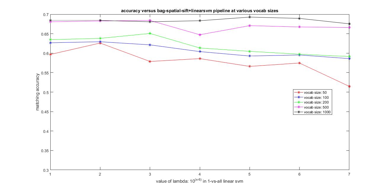
|
Clearly, adding spatial information by using level-2 Spatial-Bag-of-Sift+SVM has improved the accuracy compared to the plain Bag-of-Sift+SVM pipeline. The best possible accuracy with this Spatial-Bag-of-features+SVM pipeline achieved was around 68.1% using vocab_size=1000 and lambda=0.1
I have also calculated the accuracy and the confusion matrix using the bags_sift_spatial_features model and the values of the paramaters used: step equal to 4, size equal to 16,fast, sampled all the features and level=1, for get_spatial_bags_of_sifts using a vocabulary of size 500 and value of the parameter lambda = 0.001 in Linear SVM. Following are the results using this parameters.
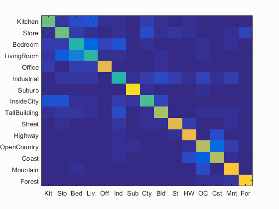
Accuracy (mean of diagonal of confusion matrix) is 0.683 with the values of the paramaters used: step equal to 4, size equal to 16,fast, sampled all the features and level=1, for get_spatial_bags_of_sifts using a vocabulary of size 500 and value of the parameter lambda = 0.001 in Linear SVM.
Level0: meaning- using level0features
Level1: meaning- using level0+level1features
Level2: meaning- using level0+level1+level2features
Using level-2 over level-1 increases the computation time, but helps us save more spatial information and hence we get slightly better performance in level-2 over level-1. You can clearly imitate all the results sing different vocab sizes for level-1 spatial-bag-of-sift features, by just passing level=1 in the code. Hence, no further results of using level-1 are shown. I used level-2 for further experiments
I have used the following algorithm for scene recognition using Bag of Soft Spatial Sift features and k-nearest neighbors for classification.
1. Extract SIFT features for each training image (used parameter values: step equal to 4 and size equal to 16, fast). Using all the SIFT features (used all the samples here) for each image and construct a vocabulary of vocab_size using kmeans. This is a one-time operation and the vocabulary is saved then for later runs.
2. Extract SIFT features for each training and testing image (used paramaters: step equal to 4, size equal to 16,fast) and then construct Histogram of SIFT features by voting a weight inversely proportional to the distance from each cluster center to that particular cluster for each SIFT feature. Construct this histogram by using a sample of features obtained from that particular image(here sampled all the feature vectors from each image for constructing the histogram of that particular image for good performance).
3. level-1: Now repeat the step2 by dividing the image into 2x2 and extract histograms for each sub-part of the image, so we will obtain 4 additional histograms now.
4. level-2: Now again repeat step2 by dividing the original image into 4x4 and extract hostograms for each of these sub-parts. We will have 16 histograms at this level.
5. two ways to implement this: use level-0 and level-1 features: concatenate them and use them as features
(or) use level-0, level-1 and level-2 features: concatenate them and then use them as features.
6. Obtain such histogram for each training and testing image and now these are to used as Features for the next steps.
7. For each test image, obtain the feature of the image as described above and used K-nearest neighbors and assign the majority label among the K-nearest neighbors found using the euclidean distance metric.
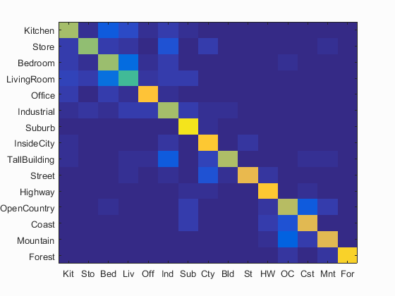
I have calculated the accuracy and the confusion matrix using the bags_sift_spatial_soft_features model and the values of the paramaters used: step equal to 4, size equal to 16,fast and sampled all features, used vote=10000/distance, used level=2 for get_spatial_bags_of_sifts_soft using a vocabulary of size 1000 and value of the parameter K=8 in K-nearest neighbors. Following are the results using this parameters.
Accuracy (mean of diagonal of confusion matrix) is 0.539 with the values of the paramaters used: step equal to 4, size equal to 16,fast and sampled all features, used vote=10000/distance, used level=2 for get_spatial_bags_of_sifts_soft using a vocabulary of size 1000 and value of the parameter K=8 in K-nearest neighbors.
Following is an analysis of the various parameters involved in this pipeline. I have tried varying the vocabulary size from 50,100, 200, 500 and 1000. I have always used the same paramters for the sift features: step-4,size-16,'fast',level=2,vote=10000/distance. I used all the features from the training and testing images to construct their histogram which is used as features and the value of K varying from 1 to 30 in k-nearest neighbors.
Observations:
1. As I increased the vocabulary size, the time taken is increasing slightly but here there was no clear improvement of performance as you can see from the plot below.
2. As I increased the value of K in k-nearest neighbors, the time taken has reduced to compute the predicted label for each image and there was not much of improvement in performance although it did help in a few cases.
The image below shows the results of accuracy versus the vocabulary size from 50,100, 200, 500 and 1000 and using all the features from the training and testing images to construct their histogram which is used as features and the value of K varying from 1 to 30 in k-nearest neighbors.
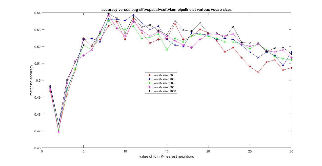
|
Using kernel book encoding, adding spatial information by using level-2 Soft-Spatial-Bag-of-Sift+KNN has not improved the accuracy compared to the Spatial Bag-of-Sift+KNN pipeline, but dropped slightly. The best possible accuracy with this Soft-Spatial-Bag-of-features+KNN pipeline achieved was around 53.9% using vocab_size=1000 and k=8
I have used the following algorithm for scene recognition using Bag of Soft Spatial Sift and SVM for classification.
1. Extract SIFT features for each training image (used parameter values: step equal to 8 and size equal to 16,fast). Using all the SIFT features (used all the samples here) for each image and construct a vocabulary of vocab_size using kmeans. This is a one-time operation and the vocabulary is saved then for later runs.
2. Extract SIFT features for each training and testing image (used paramaters: step equal to 4, size equal to 16, fast) and then construct Histogram of SIFT features by voting a weight inversely proportional to the distance from each cluster center to that particular cluster for each SIFT feature. Construct this histogram by using a sample of features obtained from that particular image(here sampled all the feature vectors from each image for constructing the histogram of that particular image for good performance).
3. Obtain such histogram for each training and testing image and now these are to used as Features for the next steps.
4. Using the features of the training data, train a 1-vs-all linearSVMs for each category which will be later used while testing.
5. For each test image, obtain the features of the images as described above and used 1-vs-all linear SVMs for each category separately and choose the label with maximum confidence.
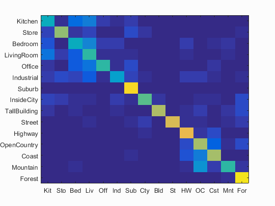
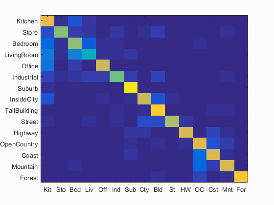
I have calculated the accuracy and the confusion matrix using the bags_sift_spatial_soft_features model and the values of the paramaters used: step equal to 4, size equal to 16,fast, sampled all the features and level=2, vote=10000/distance for get_spatial_bags_of_sifts_soft using a vocabulary of size 1000 and value of the parameter lambda = 0.00001 in Linear SVM. Following are the results using this parameters.
Accuracy (mean of diagonal of confusion matrix) is 0.752 with the values of the paramaters used: step equal to 4, size equal to 16,fast, sampled all the features and level=2, vote=10000/distance for get_spatial_bags_of_sifts_soft using a vocabulary of size 1000 and value of the parameter lambda = 0.00001 in Linear SVM.
Following is an analysis of the various parameters involved in this pipeline. I have tried varying the vocabulary size from 50,100, 200, 500 and 1000. I have always used the same paramters for the sift features: step-4,size-16,'fast',level=2,vote=10000/distance. I used all the features from the training and testing images to construct their histogram which is used as features values of lambda in SVM varying from 0.00001, 0.0001, 0.001, 0.01, 0.1, 1 and 10.
Observations:
1. As I increased the vocabulary size, although the time taken is increasing slightly, the accuracy is also improving as you can see from the plot below.
2. As I increased the value of lambda value, the time taken has reduced to compute the predicted label for each image and the performance improved in a few cases and dropped in a few. There was no clear pattern observed.
The image below shows the results of accuracy versus the vocabulary size from 50,100, 200, 500 and 1000 and using all the features from the training and testing images to construct their histogram which is used as features and the value of of lambda varying from 0.00001, 0.0001, 0.001, 0.01, 0.1, 1 and 10 in linear SVM.
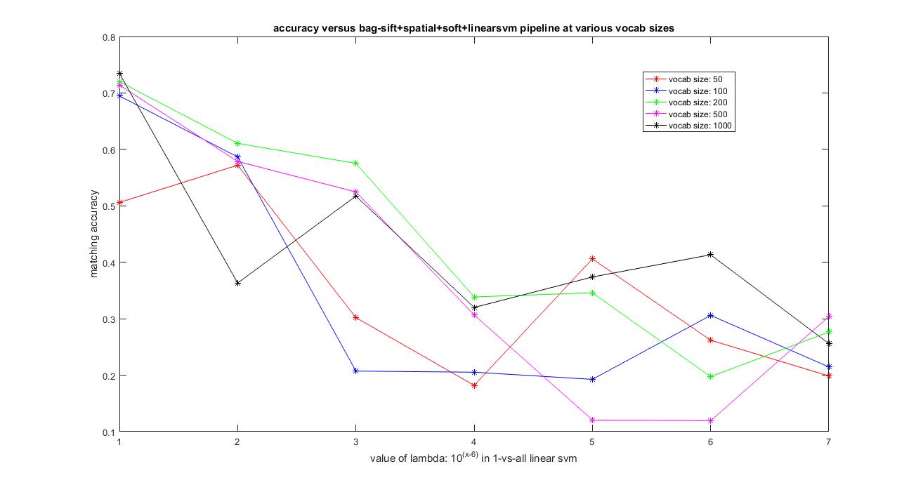
|
Clearly, here using kernel book encoding and adding spatial information by using level-2 Soft-Spatial-Bag-of-Sift+SVM has improved the accuracy compared to the previous models. The best possible accuracy with this Soft-Spatial-Bag-of-features+SVM pipeline achieved was around 75.2% using vocab_size=1000 and lambda=0.00001
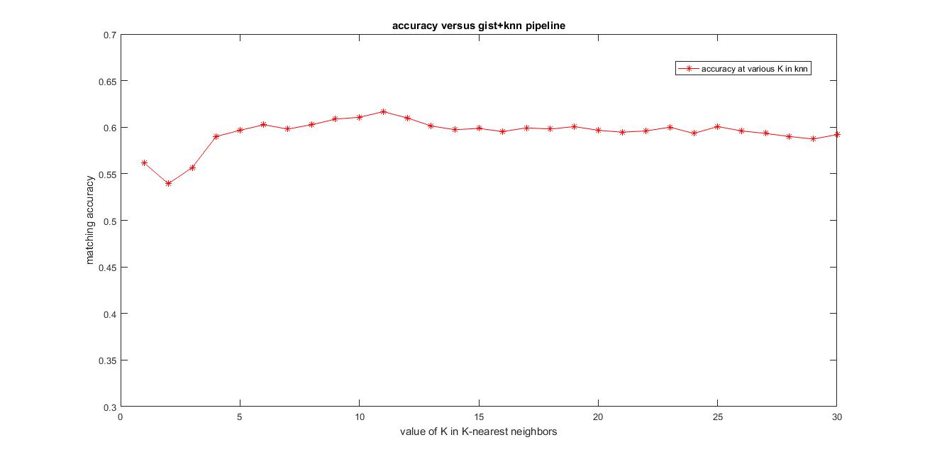
I have used the following algorithm for scene recognition using GIST features and k-nearest neighbors for classification.
1. Extract GIST for each image and use them directly as features.
2. Obtain such features for each training and testing image. Now these are to used as Features for the next steps.
3. For each test image, obtain the feature of the image as described above and used K-nearest neighbors and assign the majority label among the K-nearest neighbors found using the euclidean distance metric. (used K=11)
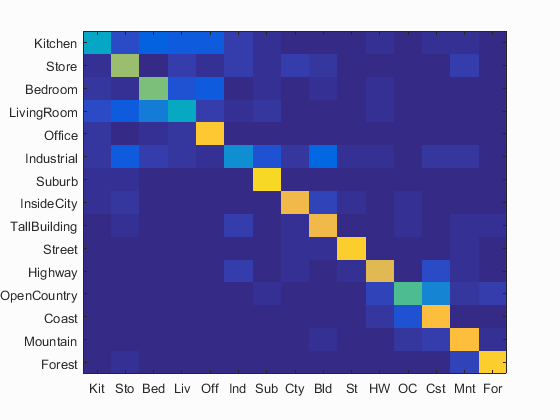
I have calculated the accuracy and the confusion matrix using the gist features and the values of paramters used are: param.imageSize = [256 256], param.orientationsPerScale = [8 8 8 8], param.numberBlocks = 4, param.fc_prefilt = 4 in get_gist_features,k=11. Following are the results using this parameters.
Accuracy (mean of diagonal of confusion matrix) is 0.617 with the values of paramters used are: param.imageSize = [256 256], param.orientationsPerScale = [8 8 8 8], param.numberBlocks = 4, param.fc_prefilt = 4 in get_gist_features,k=11.
Using GIST features+KNN has improved the accuracy compared to the previous methods. Accuracy obtained here is 61.7%
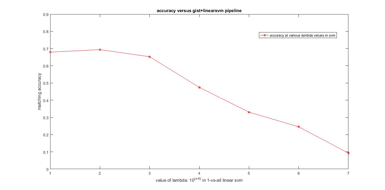
I have used the following algorithm for scene recognition using GIST features and svm for classification.
1. Extract GIST for each image and use them directly as features.
2. Obtain such features for each training and testing image. Now these are to used as Features for the next steps.
3. For each test image, obtain the features of the images as described above and used 1-vs-all linear SVMs for each category separately and choose the label with maximum confidence.
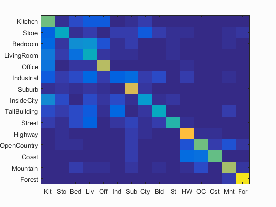
I have calculated the accuracy and the confusion matrix using the gist features model and the values of the paramaters used are: param.imageSize = [256 256], param.orientationsPerScale = [8 8 8 8], param.numberBlocks = 4, param.fc_prefilt = 4 in get_gist_features,lambda=0.0001. Following are the results using this parameters.
Accuracy (mean of diagonal of confusion matrix) is 0.69.9 with the values of the paramaters used are: param.imageSize = [256 256], param.orientationsPerScale = [8 8 8 8], param.numberBlocks = 4, param.fc_prefilt = 4 in get_gist_features,lambda=0.0001.
Clearly, using GIST features has improved the accuracy compared to the plain bag of sifts model. Accuracy obtained here is 69.9%
I have used the following algorithm for scene recognition using GIST+Bag of Soft Spatial Sift features and k-nearest neighbors for classification.
1. Extract SIFT features for each training image (used parameter values: step equal to 4 and size equal to 16, fast). Using all the SIFT features (used all the samples here) for each image and construct a vocabulary of vocab_size using kmeans. This is a one-time operation and the vocabulary is saved then for later runs.
2. Extract SIFT features for each training and testing image (used paramaters: step equal to 4, size equal to 16,fast) and then construct Histogram of SIFT features by voting a weight inversely proportional to the distance from each cluster center to that particular cluster for each SIFT feature. Construct this histogram by using a sample of features obtained from that particular image(here sampled all the feature vectors from each image for constructing the histogram of that particular image for good performance).
3. level-1: Now repeat the step2 by dividing the image into 2x2 and extract histograms for each sub-part of the image, so we will obtain 4 additional histograms now.
4. level-2: Now again repeat step2 by dividing the original image into 4x4 and extract hostograms for each of these sub-parts. We will have 16 histograms at this level.
5. two ways to implement this: use level-0 and level-1 features: concatenate them and use them as features
(or) use level-0, level-1 and level-2 features: concatenate them and then use them as features.
6. Obtain such histogram for each training and testing image and concatenate them with GIST features. Now these are to used as Features for the next steps.
7. For each test image, obtain the feature of the image as described above and used K-nearest neighbors and assign the majority label among the K-nearest neighbors found using the euclidean distance metric. (used K=11)
I have calculated the accuracy and the confusion matrix using the bags_sift_spatial_soft_gist_features model and the values of the paramaters used: step equal to 4, size equal to 16,fast and sampled all features, used vote=10000/distance, used level=2 for get_spatial_bags_of_sifts_soft using a vocabulary of size 1000 and value of the parameter K=11 in K-nearest neighbors. For gist paramters used are: param.imageSize = [256 256], param.orientationsPerScale = [8 8 8 8], param.numberBlocks = 4, param.fc_prefilt = 4 in get_gist_features. Following are the results using this parameters.
Accuracy (mean of diagonal of confusion matrix) is 0.538 with the values of the paramaters used: step equal to 4, size equal to 16,fast and sampled all features, used vote=10000/distance, used level=2 for get_spatial_bags_of_sifts_soft using a vocabulary of size 1000 and value of the parameter K=11 in K-nearest neighbors. For gist paramters used are: param.imageSize = [256 256], param.orientationsPerScale = [8 8 8 8], param.numberBlocks = 4, param.fc_prefilt = 4.
Using GIST features combined with kernel book encoding, adding spatial information by using level-2 GIST+Soft-Spatial-Bag-of-Sift+KNN has not improved the accuracy compared to the previous methods, but dropped slightly. Accuracy obtained here is 53.8%
I have used the following algorithm for scene recognition using GIST+Bag of Soft Spatial Sift features and SVM for classification.
1. Extract SIFT features for each training image (used parameter values: step equal to 8 and size equal to 16,fast). Using all the SIFT features (used all the samples here) for each image and construct a vocabulary of vocab_size using kmeans. This is a one-time operation and the vocabulary is saved then for later runs.
2. Extract SIFT features for each training and testing image (used paramaters: step equal to 4, size equal to 16, fast) and then construct Histogram of SIFT features by voting a weight inversely proportional to the distance from each cluster center to that particular cluster for each SIFT feature. Construct this histogram by using a sample of features obtained from that particular image(here sampled all the feature vectors from each image for constructing the histogram of that particular image for good performance).
3. Obtain such histogram for each training and testing image and concatenate them with GIST features. Now these are to used as Features for the next steps.
4. Using the features of the training data, train a 1-vs-all linearSVMs for each category which will be later used while testing.
5. For each test image, obtain the features of the images as described above and used 1-vs-all linear SVMs for each category separately and choose the label with maximum confidence.
I have calculated the accuracy and the confusion matrix using the bags_sift_spatial_soft_gist_features model and the values of the paramaters used: step equal to 4, size equal to 16,fast, sampled all the features and level=2, vote=10000/distance for get_spatial_bags_of_sifts_soft using a vocabulary of size 1000 and value of the parameter lambda = 0.00001 in Linear SVM. For gist paramters used are: param.imageSize = [256 256], param.orientationsPerScale = [8 8 8 8], param.numberBlocks = 4, param.fc_prefilt = 4 in get_gist_features. Following are the results using this parameters.
Accuracy (mean of diagonal of confusion matrix) is 0.729 the values of the paramaters used: step equal to 4, size equal to 16,fast, sampled all the features and level=2, vote=10000/distance for get_spatial_bags_of_sifts_soft using a vocabulary of size 1000 and value of the parameter lambda = 0.00001 in Linear SVM. For gist paramters used are: param.imageSize = [256 256], param.orientationsPerScale = [8 8 8 8], param.numberBlocks = 4, param.fc_prefilt = 4 in get_gist_features.
Clearly, using GISTfeatures and combining with using kernel book encoding and adding spatial information by using level-2 GIST+Soft-Spatial-Bag-of-Sift+SVM has not improved the accuracy compared to the previous model, but dropped slightly. Accuracy obtained here is 72.9%
All the work that has been implemented for the project has been presented and discussed above. Feel free to contact me for further queries.
Contact details:
Murali Raghu Babu Balusu
GaTech id: 903241955
Email: b.murali@gatech.edu
Phone: (470)-338-1473
Thank you!