Jatin Nanda

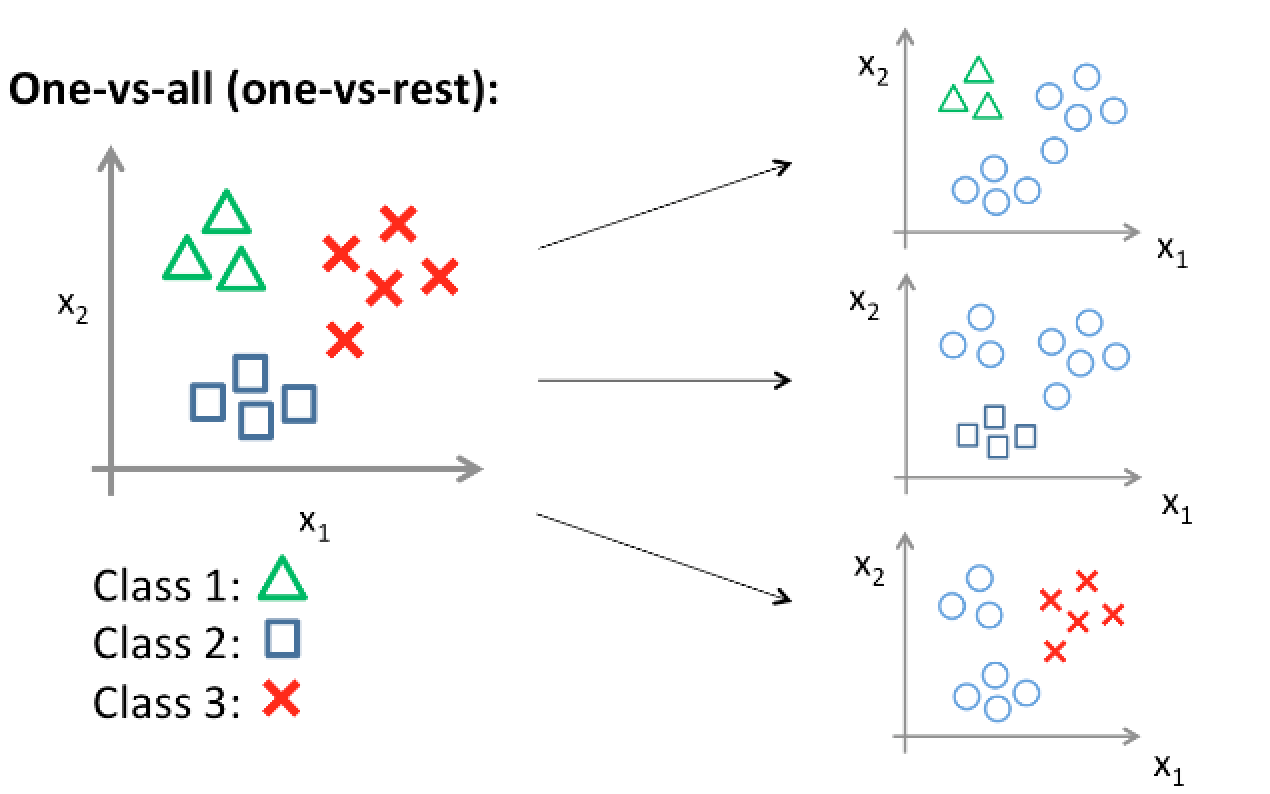
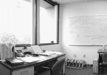
Above is an illustration of a 1-vs All SVM classifier

Tiny Images Descriptor

The tiny images descriptor was performed as a naive attempt at describing an image. It works by shrinking the image to a 16x16 pixels. Once this image is scaled down (the sampling rate is reduced) and fine features of the image are lost, but more prominent ones remain. This descriptor, as one can imagine, did not produce the best results. This is largely due to its lossy nature. It is worth noting that the resulting matrix was normalized with 0 mean and unit variance to reduce the effect of size.

Nearest-Neighbor Classifier

The nearest-neighbor classifier is often thought of as one of the simplest classifiers in existence, but it's surprising how well it can do by averaging over different values of k. It is likely that an increase in the value of k would increase accuracy as the classifier would overfit less to the training data and generalize better. In my implementation, I used a simple 1-NN classifier by using vl_feat's built-in distance function. Being that it was 1-NN, no parameters had to be adjusted - all 15000 training and testing inputs were used. Below is the result of a 1-NN with an accuracy of 0.225.

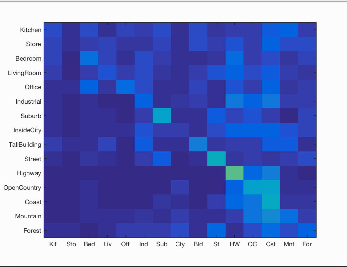
Accuracy (mean of diagonal of confusion matrix) is 0.225

Bag of SIFT Descriptor

A far better approach to describing an image relied on using a bag of SIFT descriptor. For each image, SIFT features are found using vl_feat's built-in function and are categorized into the 'visual words' with a histogram approach. For my histogram, I used weights for the top ~5 neighbors for each of the features, and I noticed a modest improvement in results. This is likely because more information about the picture is retained and less overfitting occurs (as with using a larger K value in KNN). Finally, the histogram was normalized and the result was stored appropriately. The parameter that affected performance the most significantly in this stage was the step_size of the SIFT feature extraction. With too large of a step size, the implementation would run quickly, however the accuracy would suffer tremendously. This is because we are effectively reducing the sampling rate and losing information from the image that may be vital to accurate classification. Increasing the number of features extracted from each image also improved the results by 2-3%. Additionally, the 'fast' flag was turned off to improve performance, but no significant improvement was observed. All in all, this SIFT descriptor approach was able to improve my accuracy with a simple 1-NN to 0.539!

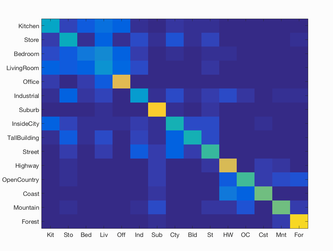
Accuracy (mean of diagonal of confusion matrix) is 0.539

Linear SVM Classifier

The last phase of this project involved moving from the nearest-neighbors classifier to a linear SVM. A linear SVM seeks to create a decision boundary represented by a linear function on the data, but unfortunately only works with two classes. To create a multi-class SVM, I employed the 1-vs all approach and created one SVM for each category and reported the winning categories. With this classifier, the biggest parameter that affected results was lambda. Lambda represents the level of regularization the classifier should have, and with my results, it seemed that a generally lower level of lambda resulted in higher test-accuracies. This is largely in part due to the fact that with larger values of lambda (1, 10) the model would overfit the training data and perform terribly on the testing data. The optimal lambda I found was 0.0001, which resulted in an accuracy of 0.694!

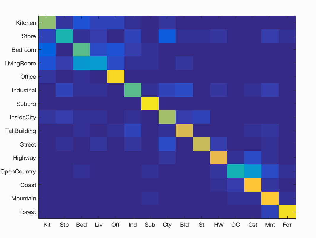
Accuracy (mean of diagonal of confusion matrix) is 0.694

Category name	Accuracy	Sample training images		Sample true positives		False positives with true label		False negatives with wrong predicted label
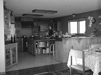
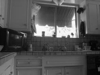
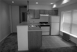
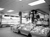
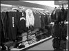
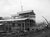
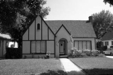
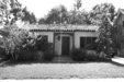
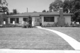
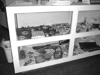
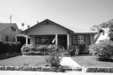
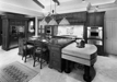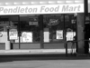
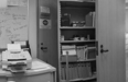
Kitchen	0.630					Store	Store	Office	LivingRoom
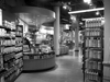
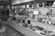
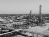
Store	0.460					Industrial	LivingRoom	LivingRoom	InsideCity
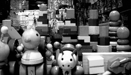
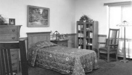
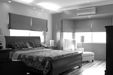
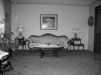
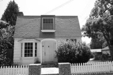
Bedroom	0.560		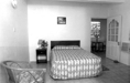			Office	Kitchen	LivingRoom	Suburb
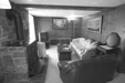
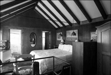
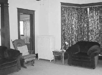
LivingRoom	0.330		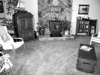			Kitchen	Store	Store	Suburb
Office	0.910					LivingRoom	Bedroom	Bedroom	Kitchen
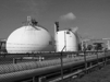
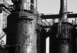
Industrial	0.550		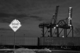			LivingRoom	TallBuilding	Coast	TallBuilding
Suburb	0.940		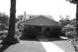			Store	Office	Coast	Industrial
InsideCity	0.670					Store	Store	Industrial	Street
TallBuilding	0.760					Mountain	Industrial	Coast	Bedroom
Street	0.720					InsideCity	Store	InsideCity	InsideCity
Highway	0.790					OpenCountry	InsideCity	Mountain	Coast
OpenCountry	0.450					Mountain	Industrial	Coast	Mountain
Coast	0.850					OpenCountry	OpenCountry	OpenCountry	Highway
Mountain	0.860					OpenCountry	Forest	Coast	OpenCountry
Forest	0.930					OpenCountry	Highway	Mountain	Mountain
Category name	Accuracy	Sample training images		Sample true positives		False positives with true label		False negatives with wrong predicted label