Project 3: Camera Calibration and Fundamental Matrix Estimation with RANSAC
Contents
- Camera Projection Matrix
- Fundamental Matrix Estimation
- Fundamental Matrix with RANSAC
- Extra credit/Graduate credit
1. Camera Projection Matrix
Camera projection matrix mps 2D world coordinates to image coordinates. To estimate the projection matrix, corresponding 3D and 2D points in one image need to be provided.
From the homogeneous transformation equation,
we can derive a system of equations as follows, taking all the elements in the projection matrix as unknown variables.
As the projection matrix has only 11 degrees of freedom and 1 scaling variable, the last element in the homogeneous transformation is set to be 1.
By using matlab
A\b operation, we solve the system of linear equations in the least square sense.
Reformulate the projection matrix into 3x4 matrix form. The result from the provided 3D and 2D points is,
The matrix is exactly a scaled equivalent of the correct one. Using the projection Matrix to map the 3D points back to 2D coordinate plane, we can compare the actual 2D points and projected 2D points in the following figure.
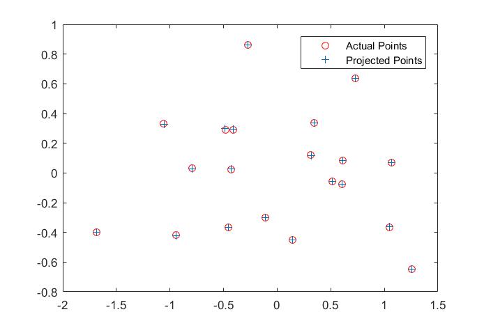
Fig. 1 Projected results
With the projection matrix, we can decompose it and find the camera center as,
We can also map the camera and all points in 3D using the provided function, along with the actual image as a side comparason.
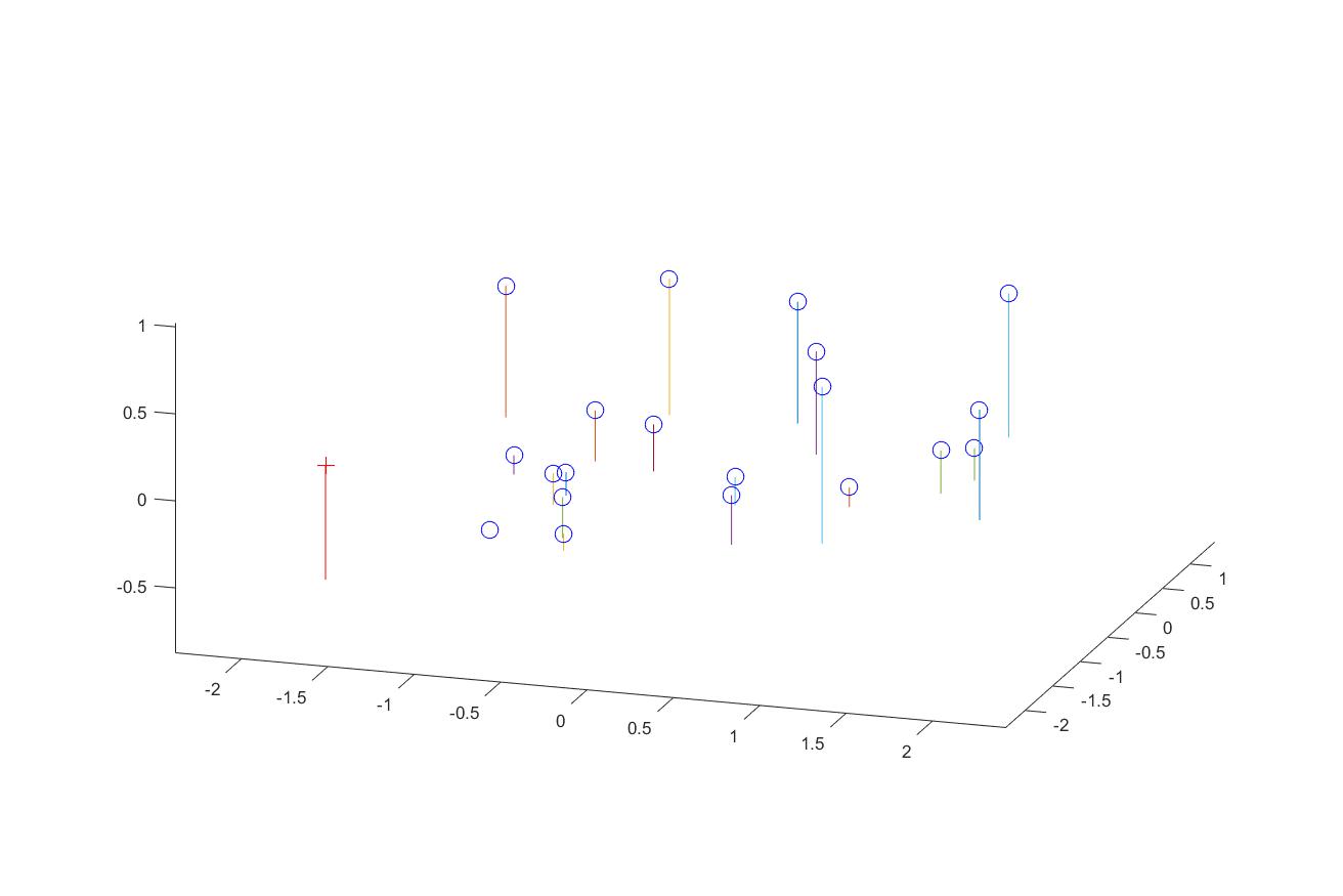
Fig. 2 3D visulization of the points and camera
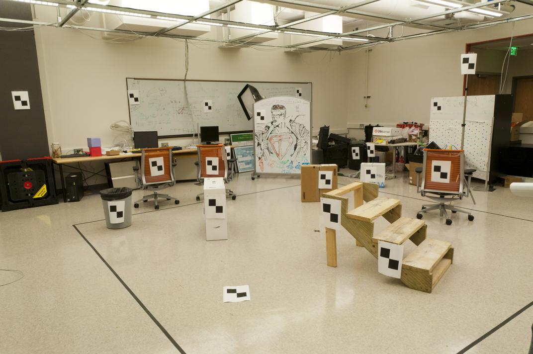
Fig. 3 Original image
2. Fundamental Matrix Estimation
The fundamental matrix relates points in one scene to epipolar lines in the other scene. To estimate the fundamental matrix,
we need correspoinding 2d points across two images. The fundamental properity of the fundamental matrix is,
Expand the matrix multiplication into a scaler equation.
Similarly, we can transforma the problem into solving a system of linear equations with multiple corresponding
2D points.
With input correspoinding 2D points
Points_a and
Points_b, we can compose the matrix
A as
LinEquMatrix by the following.
LinEquMatrix = zeros(numPoints,9);
LinEquMatrix(:,1) = Points_a(:,1).*Points_b(:,1);
LinEquMatrix(:,2) = Points_a(:,2).*Points_b(:,1);
LinEquMatrix(:,3) = Points_b(:,1);
LinEquMatrix(:,4) = Points_a(:,1).*Points_b(:,2);
LinEquMatrix(:,5) = Points_a(:,2).*Points_b(:,2);
LinEquMatrix(:,6) = Points_b(:,2);
LinEquMatrix(:,7:8) = Points_a;
LinEquMatrix(:,9) = ones(numPoints,1);
Decompose the matrix A by SVD decomposition. The fundamtrix matrix
F_matrix is the last column vector of the unitary matrix.
As the fundamental matrix is of rank 2, we need to set the smallest singular value in its SVD decomposition to 0.
[U,S,V]= svd(LinEquMatrix);
Fvector = V(:,end);
F_matrix = reshape(Fvector,[3,3])';
[U,S,V] = svd(F_matrix);
S(3,3) = 0;
F_matrix = U*S*V';
Based on the estimated fundamental matrix, we can draw epipolar lines on the each image. The epipolar lines are going to cross
the correspoinding points.
Fig. 4 Epipolar Lines on the image pair
Because there are numerical errors when solving the system of linear equations, the epipolar lines are not perfectly crossing the
correspoinding points. Using normallization on all the data points (Extra credit part), we can achieve perfect alignment on the
points by reducing the numerical error on the fundamental matrix, as shown in Fig. 5. The fundamental matrix is
Fig. 5 Epipolar Lines on the image pair using Normalization on points
3. Fundamental Matrix with RANSAC
Fundamental matrix can also be used for matching features from multiple scenes. Often times perfect point corresponence from
differnt scenes does not exist. To leveage the unreliable point correspondences, RANSAC can be applied to estimate the
fundamental matrix from noisy point pairs. SIFT feature detector is used to find interest point pairs. VLFeat toolbox is
used to do SIFT matching. However VLFeat 0.9.20 binary package has compactiablity issue in Win 10 environment. VLFeat 0.9.19
is finally installed at last.
8 or more point pairs (parameter from numChosen) is iteratively randomly chosen as the input for calculating the fundamental matrix. Then inliers are found for this
fundamental matrix based on the distance measurement. If a point pair satisfies XFX'< Threshold ,
then it is count as an inlier. Choose the fundamental matrix that provides the most inliers from a certain number of iterations.
Then with experimented values of the thresold and maximum number of iterations, we can find good fundamental matrix.
There are mainly 3 parameters, namely numChosen, Threshold and numItr. Different parameters
have different effects on the results. As the matched features from VLFeat are not all right, randomly chosen numChosen pairs
from them can easily give us bad pairs for calculating the fundamental matrix. Thus we would choose less numChosen pairs to calculate
the fundamental matrix and run large number of iterations to find the best fundamental matrix calculation with maximum inliers. Thus for the following
image pairs, numChosen is generally 8 and numItr is over 2000. The thresold value is chosen so that the maximum number of
inliers are generally 1/4 of all the input matched features. It should not be too small or too large. However, with carefully chosen
parameters, the fundamental matrix found from RANSAC does not necessarily be perfect because the points are coplanar and the
cameras are not actually pinhole cameras and have lens distortions. But after testing several image pairs, it is safe to say that the
fundamental matrix from RANSAC could help remove incorrect point matches.

Fig. 6a Mount Rushmore Matched features with numChosen = 8, Threshold = 6e-4; NumIteration = 2k
Fig. 6b Epipolar lines on Mount Rushmore pair from the best fundamental matrix
Fig. 6c Epipolar lines on Mount Rushmore pair from the re-estimated fundamental matrix

Fig. 7a Matched features with numChosen = 8, Threshold = 6e-4; NumIteration = 2k
Fig. 7b Epipolar lines on Notre Dame pair from the best fundamental matrix
Fig. 7c Epipolar lines on Notre Dame pair from the re-estimated fundamental matrix

Fig. 8a Gaudi Matched features with numChosen = 8, Threshold = 8e-4; NumIteration = 20k
Fig. 8b Epipolar lines on Gaudi pair from the best fundamental matrix
Fig. 8c Epipolar lines on Gaudi pair from the re-estimated fundamental matrix
4. Extra credit/Graduate credit
As images from different scenes can be shifted and scaled, coordinate normalization improve the estimation of fundamental matrix
Scaling after linear transformation is implemented here. For each image, first all the points are shifted so that their mean
is (0,0). After that, a scaling facter is calculated so that after scaling the average distance between each point and the center (0,0)
is square root of 2.
numPoints = size(matches_a,1);
mean_a = sum(matches_a,1)/numPoints;
matches_a = matches_a - repmat(mean_a,[numPoints,1]);
scale_a = sqrt(sum(sum(matches_a.^2))/2/numPoints);
matches_a = matches_a/scale_a;
TranslationA = [1,0;0,1;0,0]';
TranslationA = [TranslationA;[-mean_a,1]]';
TransformA = diag([1/scale_a,1/scale_a,1])*TranslationA;

mean_b = sum(matches_b,1)/numPoints;
matches_b = matches_b - repmat(mean_b,[numPoints,1]);
scale_b = sqrt(sum(sum(matches_b.^2))/2/numPoints);
matches_b = matches_b/scale_b;
TranslationB = [1,0;0,1;0,0]';
TranslationB = [TranslationB;[-mean_b,1]]';
TransformB = diag([1/scale_b,1/scale_b,1])*TranslationB;
The scaling after translation defines a transformation matrix for each image, which also needs to be calculated to adjust the
fundamental matrix calculated from the normalized coordinates. With this adjustment, the fundamental matrix can operate on the
original coordinates.
F_matrix = transpose(TransformB)*F_matrix*TransformA;


