Project 3 / Camera Calibration and Fundamental Matrix Estimation with RANSAC
In this project, we estimate important image properties like the camera projection matrix and the fundamental matrix. We use RANSAC to estimate the fundamental matrix when we are given unreliable point corresopndences. Finally, we use RANSAC to improve the accuracy of SIFT correspondences.
Estimating camera projection matrix
If we are given a set of world coordinate and image coordinate pairs, we can estimate the linear transformation from the world coordinates to the image coordinates. The linear transformation is shown below with X, Y, and Z being the world coordinates, u and v being image coordinates, and s being the homogeneous scale factor.
Through some algebra, we get the linear equation for the matrix elements:
With a collection of these world and image coordinates, we take the SVD of the data matrix A and set the transformation elements to the right singular vector corresponding to the smallest singular value. This vector solves the optimization problem
which gives us the nonzero vector that most closely solves the linear equation.
I implemented this procedure in the following code:
function M = calculate_projection_matrix(points2d, points3d)

X = points3d(:,1); Y = points3d(:,2); Z = points3d(:,3);
u = points2d(:,1); v = points2d(:,2);

n = length(X);
zero = zeros(n, 1);
one = ones(n, 1);

A = [X, Y, Z, one, zero, zero, zero, zero, -u.*X, -u.*Y, -u.*Z, -u;
    zero, zero, zero, zero, X, Y, Z, one, -v.*X, -v.*Y, -v.*Z, -v];
[~, ~, V] = svd(A);
m = V(:,end);
M = reshape(m, 4, 3)';

end
From the projection matrix M, we can also infer the location of the camera lens. We define the first three columns of M as the matrix Q and the fourth column as the vector m4. Then the location C of the camera lens is
This is implemented in the code below:
function center = compute_camera_center(M)

Q = M(:, 1:3);
m4 = M(:,4);
center = -Q\m4;

end
Example
With the example dataset, we find the projection matrix and camera centers respectively are:

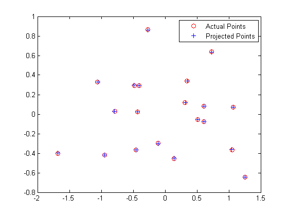
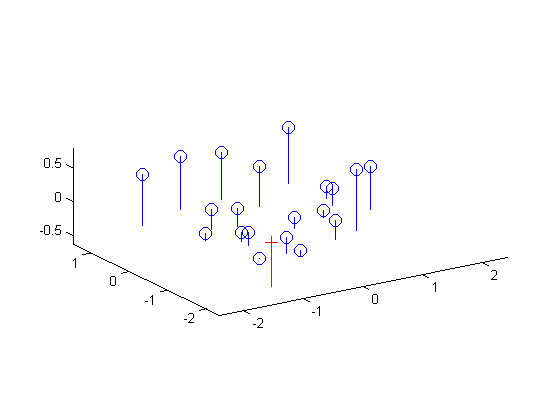
We also find that the total residual for the actual and projected image points is 0.0445. Below, the figure on the left shows these actual and predicted points, and the figure on the right shows the camera center's location along with the interest points' locations.
|
Estimating fundamental matrix
We are now given two images and interest points in both images and seek to find the mapping from a point in one image to a line in the other image. This relationship is described through the fundamental matrix F. Given a point x = (u, v, 1) in the first image and a point x' = (u', v', 1) in the second image, these two image points correspond to the same point in world coordinates if the following equation is satisfied:
Just as with the projection matrix, we solve the linear equation for a collection of points using the SVD. The matrix F we get out of it is potentially full rank though, so we set its smallest singular value to zero so that F's rank is two. This allows the epipolar lines to all intersect at the same point, the epipole.
If the values in the data matrix have a large range, our estimated F may be inaccurate due to ill-conditioning. To remedy this, for each image we center the image data at the origin by subtracting their center c and scale the points by a scalar s such that the mean squared distance between the origin and the data points is two pixels.
The scale s can be found through the following:
where each xi refers to the 2D point rather than using the homogenous coordinates. The normalized points are thus found through the following:
After we find the fundamental matrix  , we transform this matrix into one that works with our original coordinates:

where T and T' are the normalization transformations for the first and second images, respectively.
The code to find the fundamental matrix is shown below.
function F = estimate_fundamental_matrix(points_a, points_b, normalize)

n = size(points_a, 1);
one = ones(n, 1);

if nargin == 2
    normalize = true;
end

if normalize
    c_a = mean(points_a, 1);
    c_b = mean(points_b, 1);

    squared_dist_fn = @(points, c) sum(bsxfun(@minus, points, c).^2, 2);
    s_a = sqrt(2/mean(squared_dist_fn(points_a, c_a)));
    s_b = sqrt(2/mean(squared_dist_fn(points_b, c_b)));

    T_fn = @(s, c) [s*eye(2,3); 0, 0, 1]*[eye(2), -c'; 0, 0, 1];
    T_a = T_fn(s_a, c_a);
    T_b = T_fn(s_b, c_b);

    points_a = [points_a, one]*T_a';
    points_b = [points_b, one]*T_b';
else
    T_a = eye(3);
    T_b = eye(3);
end

u_a = points_a(:,1); v_a = points_a(:,2);
u_b = points_b(:,1); v_b = points_b(:,2);

A = [u_a.*u_b, u_a.*v_b, u_a, v_a.*u_b, v_a.*v_b, v_a, u_b, v_b, one];
[~, ~, V] = svd(A);
f = V(:,end);
F_fullrank = reshape(f, 3, 3);


[U, S, V] = svd(F_fullrank);
S(3,3) = 0;
F = T_b'*(U*S*V')*T_a;

end
Example
We are given the following two images along with some interest points (not shown), and we seek to find the fundamental matrix between the two.
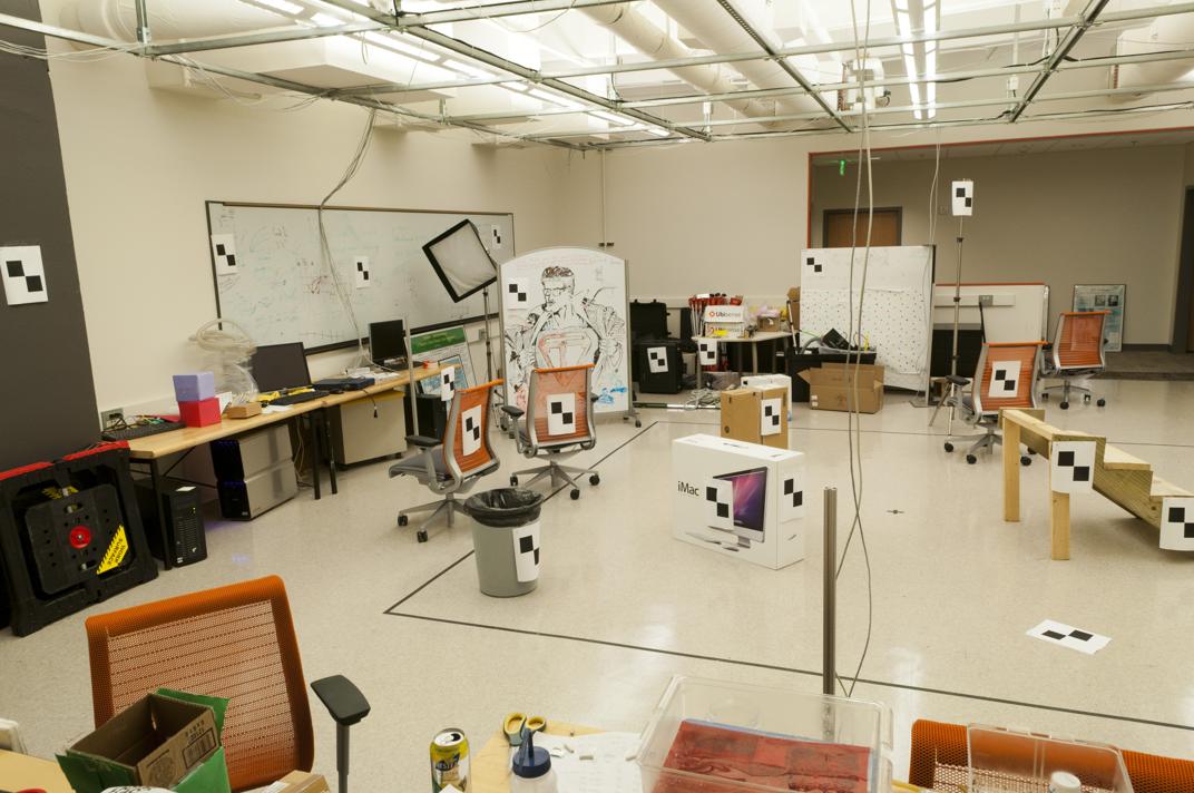
|
Without normalization, we get the epipolar lines shown below. The lines are quite accurate, but some gaps are noticeable, a symptom of poor ill-conditioning.
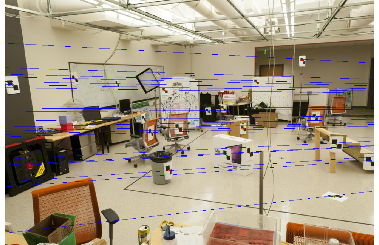

|
With normalization, we get epipolar lines that are accurate to within one pixel.
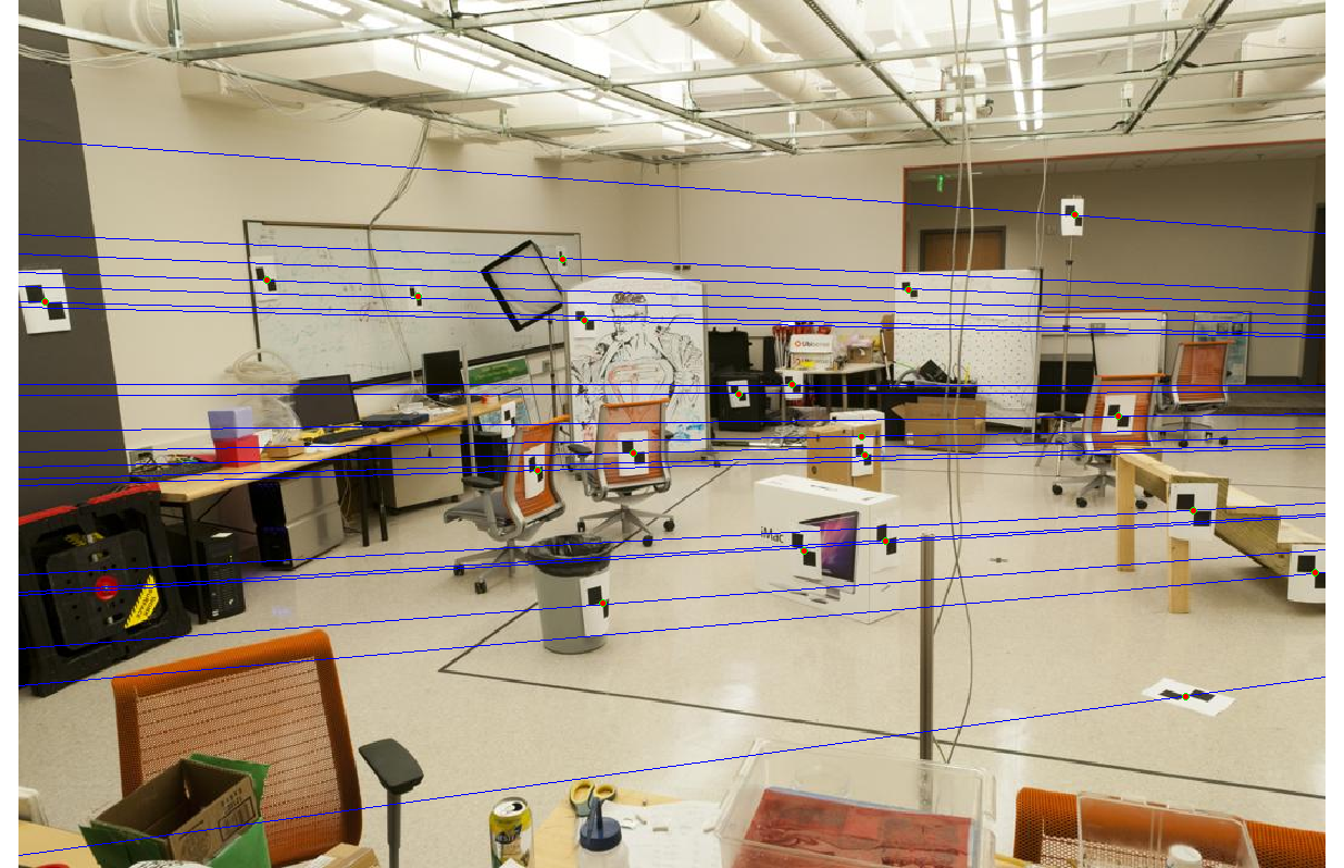

|
Even with noise added to the interest points' locations, the epipolar lines and interest points have no noticeable gaps.

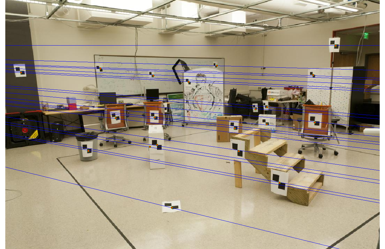
|
The three fundamental matrices are shown below. F1 corresponds to solving with the unnormalized image points, F2 to the normalized image points, and F3 to the normalized but noisy image points. The normalization appears to make a huge difference as the (3,3) element in F shifts by almost 0.8.
Estimating fundamental matrix with RANSAC
Now we must estimate the fundamental matrix just from two given images. We can use correspondences from SIFT features to estimate this matrix, but the result will be useless due to outliers. To remedy this, we rely on the RANSAC algorithm, outlined below:
- Randomly select eight pairs of points.
- Find the best fundamental matrix F from these eight pairs.
- Score this fundamental matrix by the number of inliers.
The above is repeated for some iterations, and the matrix with the highest score is returned. A pair of points (x, x') is an inlier if the distance in pixels between each point and its epipolar line is within some threshold. To be more precise, let ℓ = FTx' = (a, b, c) be the vector corresponding to the epipolar line for x', the set of all points x satisfying ℓTx = 0. The distance between some point x0 = (u0, v0) and the line ℓTx = 0 is:
We also similarly define ℓ' = Fx. We say that (x, x') is an inlier if distance(ℓ, x) and distance(ℓ', x') is less than some threshold ε. We do 50,000 iterations of the RANSAC loop to find the best model, which ensures a 99% success rate when at most 70% of the point pairs are outliers. The RANSAC code is shown below.
function [best_F, inliers_a, inliers_b] = ransac_fundamental_matrix(matches_a, matches_b)

rng(0);
ransac_iters = 5e4;
ransac_eps = 0.5;

n = size(matches_a, 1);
best_n_inliers = 0;
for i = 1:ransac_iters
    indices = randsample(n, 8);
    F = estimate_fundamental_matrix(matches_a(indices,:), matches_b(indices,:));
    [distances_a, distances_b] = get_distances(matches_a, matches_b, F);
    inliers = (distances_a <= ransac_eps & distances_b <= ransac_eps);
    if sum(inliers) > best_n_inliers
        best_n_inliers = sum(inliers);
        inliers_a = matches_a(inliers,:);
        inliers_b = matches_b(inliers,:);
        best_F = F;
    end
end

end

function [distances_a, distances_b] = get_distances(matches_a, matches_b, F)

% Returns distances from matches_a to epipolar lines in image A and
% distances from matches_b to epipolar lines in image B.

n = size(matches_a,1);
matches_a_hom = [matches_a, ones(n,1)];
matches_b_hom = [matches_b, ones(n,1)];

lines_a = matches_b_hom*F;
distances_a = distance_fn(lines_a, matches_a_hom);

lines_b = matches_a_hom*F';
distances_b = distance_fn(lines_b, matches_b_hom);

end

function distances = distance_fn(lines, points)

% Returns distances from points to corresponding lines.

dot_products = sum(lines.*points, 2);
distances = abs(dot_products) ./ sqrt(sum(lines(:,1:2).^2, 2));

end
Examples
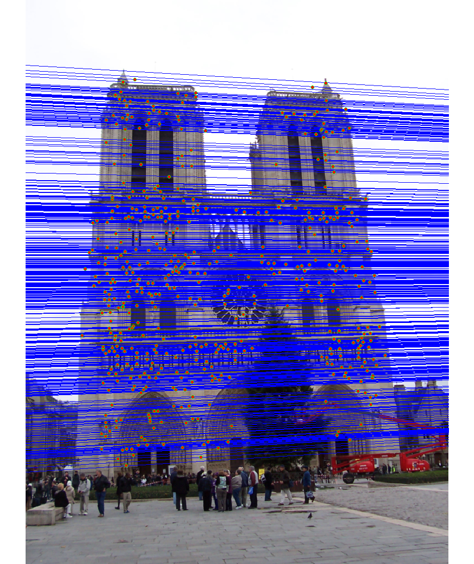
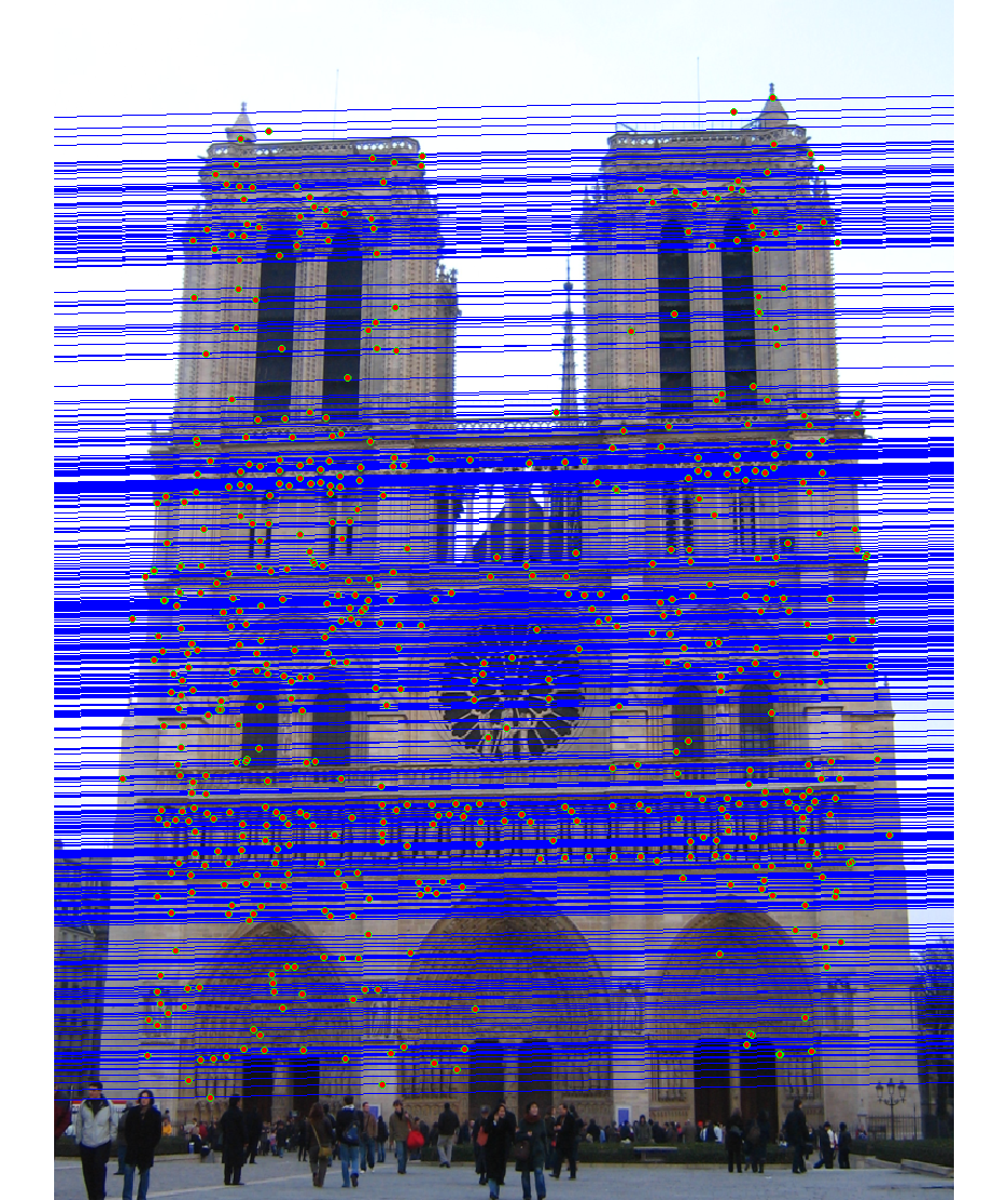
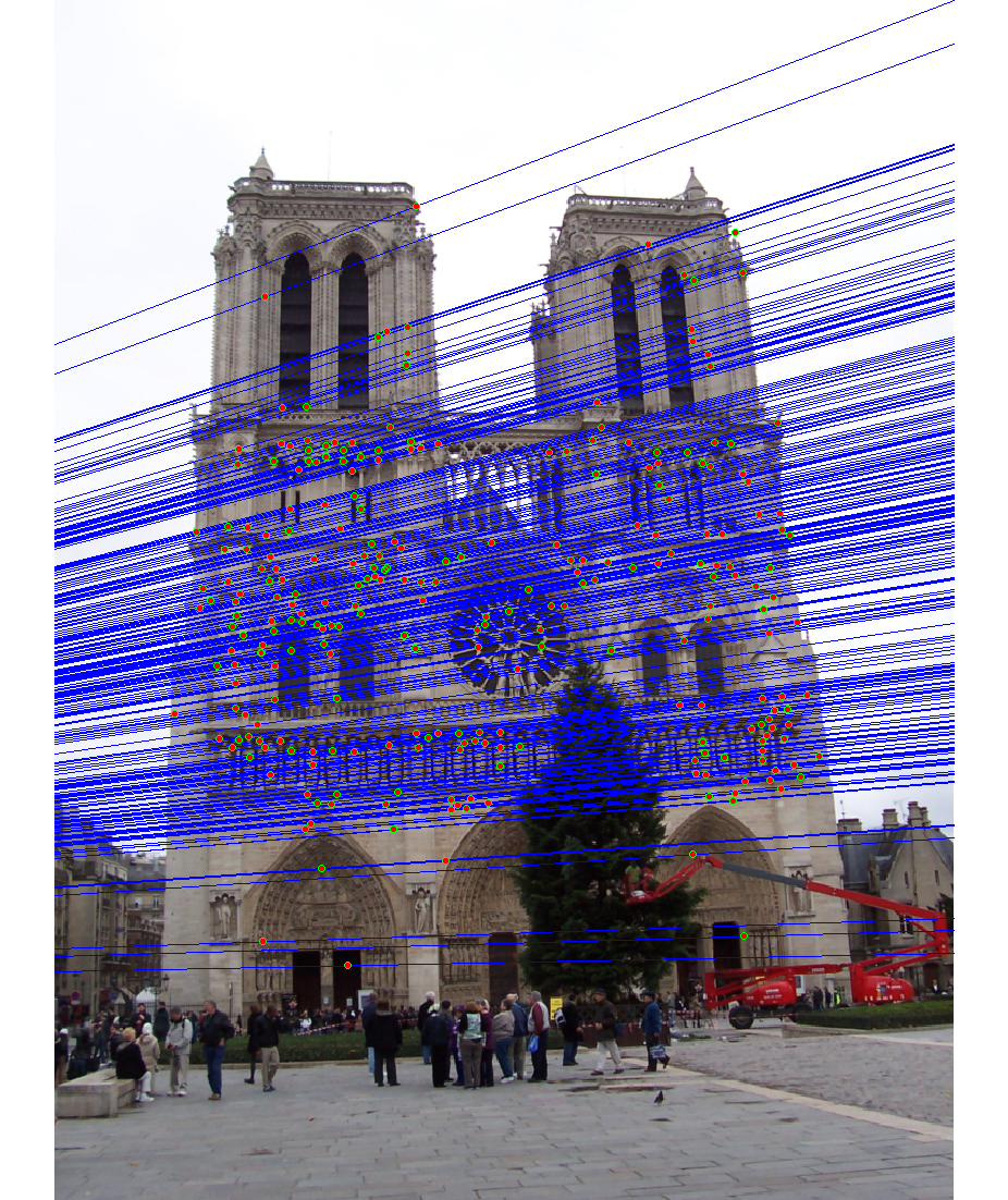
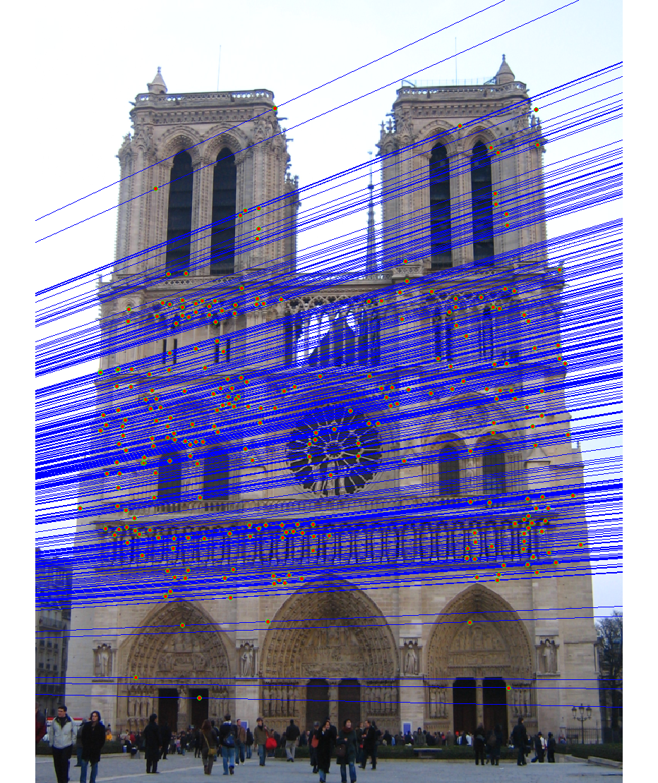
We run the algorithm on pairs of images showing Notre Dame, Mt. Rushmore, and Episcopal Goudi. The value for the inlier threshold (ransac_eps in the ransac_fundamental_matrix function) has a dramatic effect on the epipolar lines. On the Notre Dame images, setting ε to 2 pixels causes the epipolar lines to intersect at sensible locations but runs the risk of including outliers. Setting ε to half a pixel causes the epipolar lines to intersect to the left of both images, which doesn't match reality (both cameras cannot be to the left of each other). This does, however, result in much fewer outliers and might be desirable for high correspondence accuracy. The epipolar lines for both settings of ε are shown below.
|
|
|
|
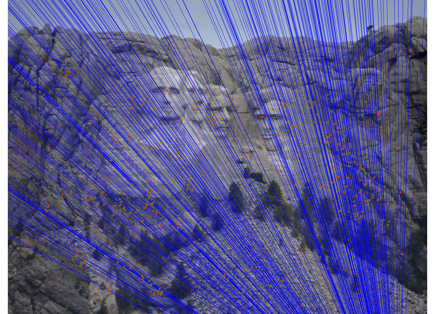
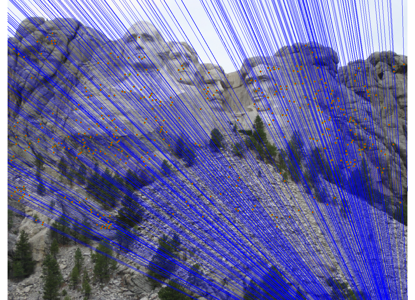
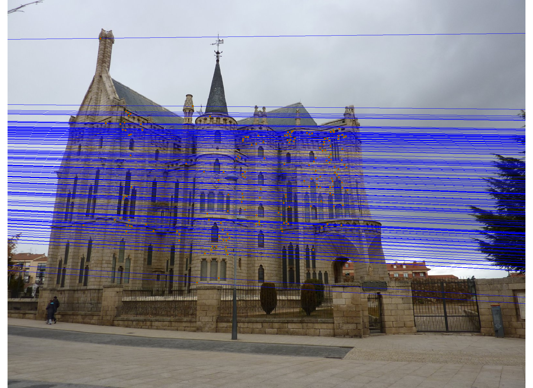
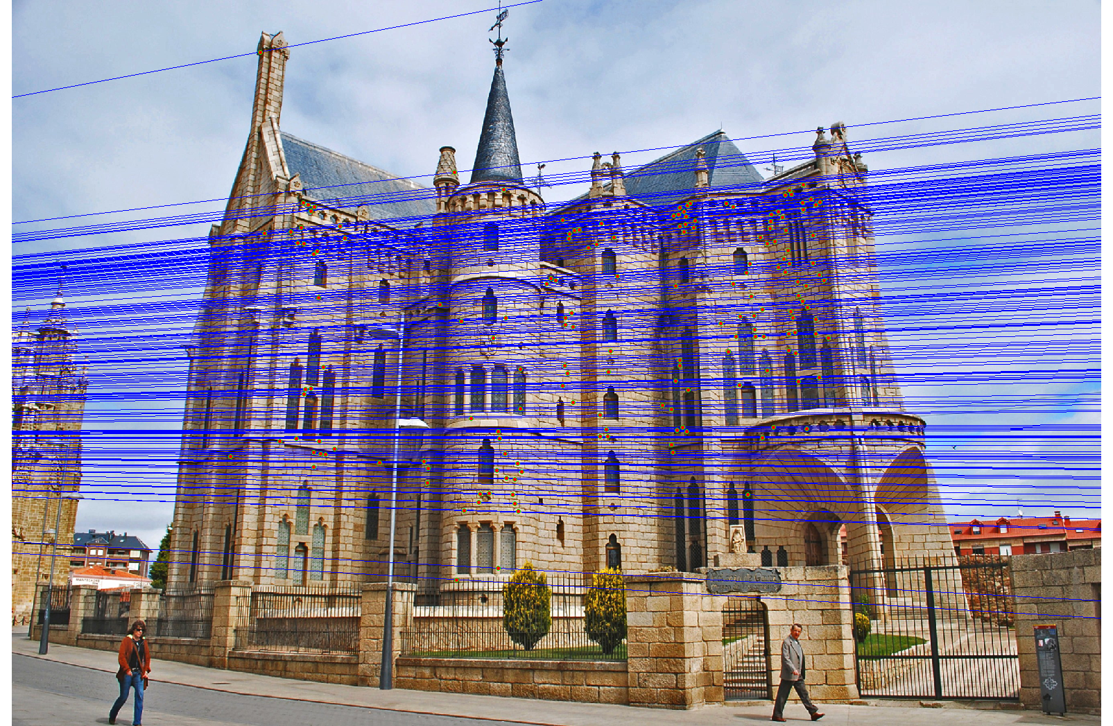
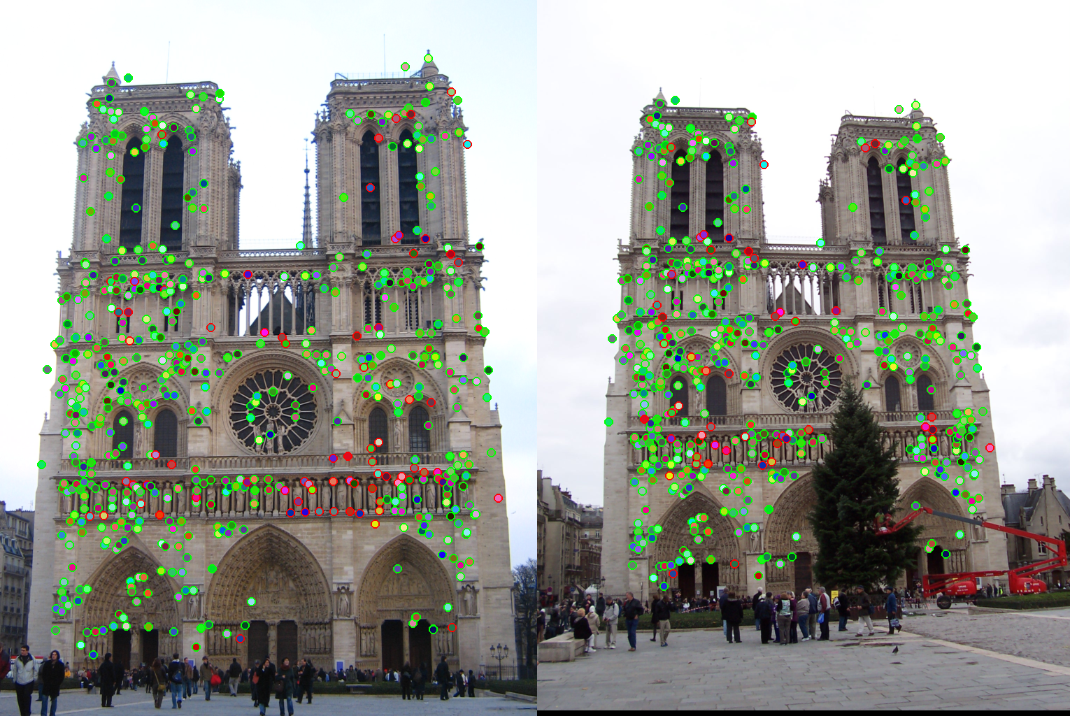
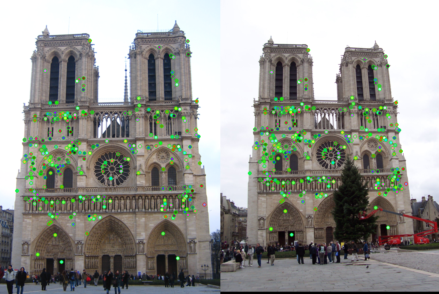
We also test RANSAC's effectiveness at selecting inliers by using the images and correspondence code from Project 2. For each image from Project 2, we scale the images by 50%. We compare the correspondence accuracy when varying the inlier threshold ε and include as a baseline the correspondence accuracy when using all the SIFT correspondences.
For each setting, each value for ε causes better correspondence accuracy than the baseline, as shown in the table below. However, there is no consistent trend between the inlier threshold and correspondence accuracy.
| No RANSAC | ε = 0.5 | ε = 1 | ε = 2 | |
| Notre Dame | 66.27% | 99.64% | 95.02% | 86.44% |
| Mt. Rushmore | 84.32% | 95.93% | 95.51% | 95.89% |
| Episcopal Gaudi | 23.20% | 64.29% | 77.27% | 90.32% |
As an example, the correspondences along with correctness color for ε set to 0.5 and 2 are shown for the Notre Dame images.
|
|